Module 14 R Markdown
Module learning objectives:
Integrate data analysis code and prose in one document
Use basic formatting for prose
Use code chunks in R to read data in, and draw tables and plots
14.1 Creating a new R Markdown file
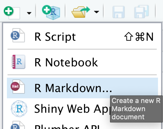
To create a new R Markdown file, click on New File then choose R Markdown...
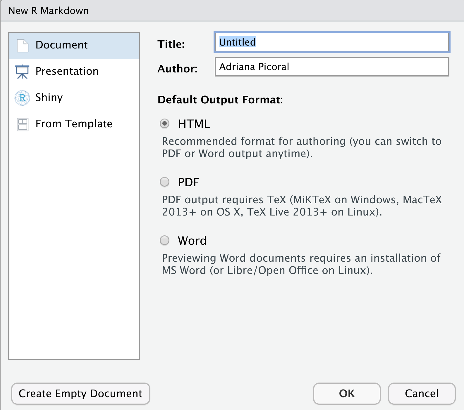
Add a title to your document (no need to change anything else). We are outputting a HTML file. To output other formats, you need to install other software.
The extension for R Markdown files is .Rmd and when you create a new file, it looks like this:
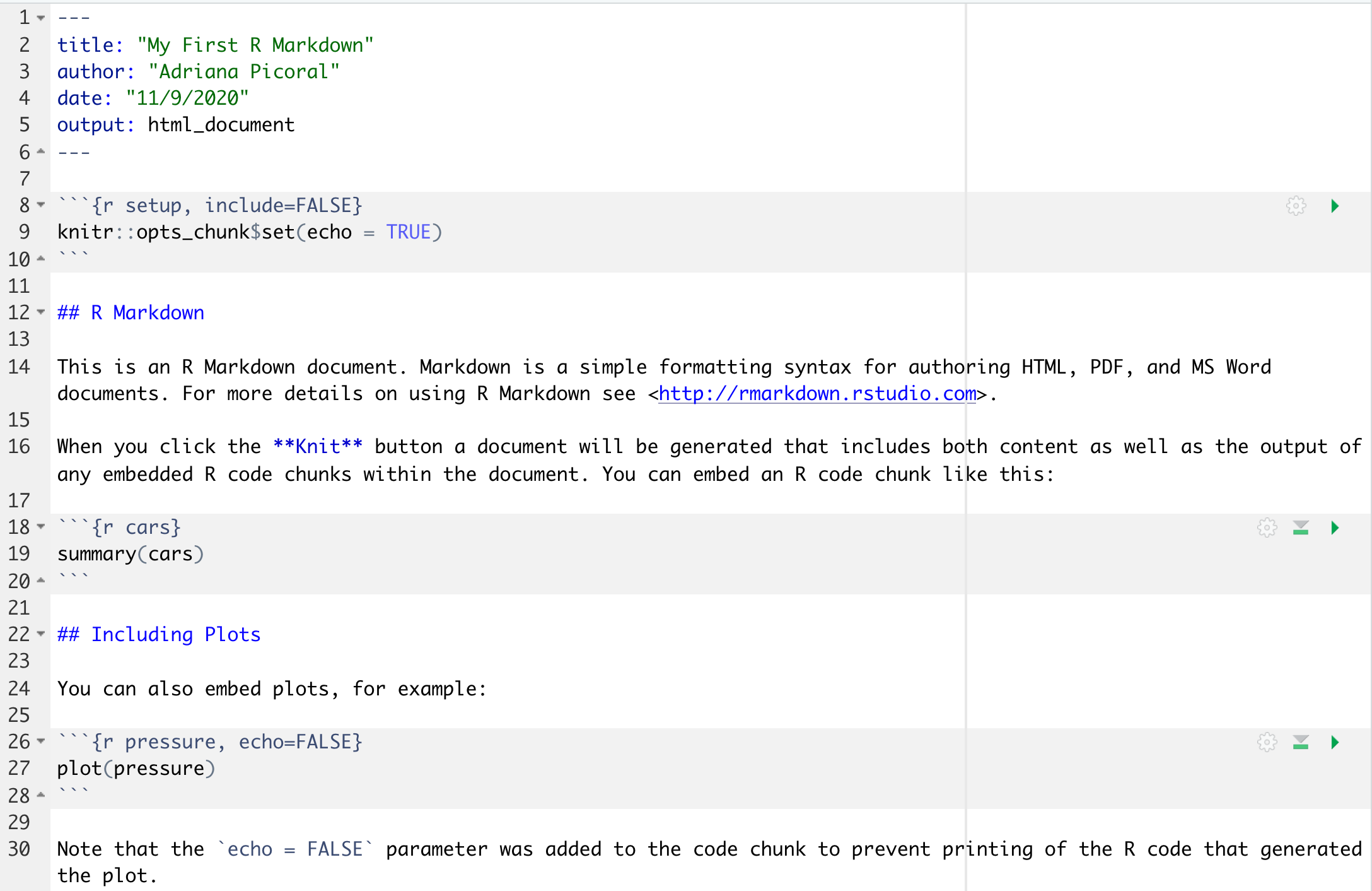
The first few lines in your new R Markdown file is an YAML header beginning and ending with ---. R code blocks start and end with ```, and the language for the code block is in between curly brackets. Note also that the text contains simple markdown formatting (e.g., # for headers and stars for bold text).
To knit your R Markdown, click on the knit icon at the top of your file panel.
![]()
14.2 Chunk Options
You can change or add knitr options for code chunks, here are some examples:
include = FALSE/TRUE: sets whether results appear in the finished file. R Markdown runs the code in the chunk regardless of boolean, and the results can be used by other chunks.
echo = FALSE/TRUE: sets whether code, but not the results, appear in the finished file.
message = FALSE/TRUE: sets whether messages that are generated by code appear in the finished file.
warning = FALSE/TRUE: sets whether warnings that are generated by code appear in the finished.
fig.cap = “…” adds a caption to graphical results.
You can check this R Markdown Reference Guide for a complete list of knitr chunk options.
14.3 Change YAML header
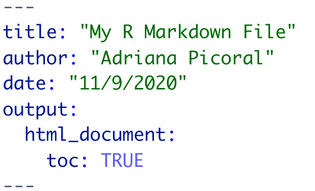
You can add a table of contents to the top of your document by changing the YAML header like so:
For more options for YAML header options check this book chapter
14.4 Text Formatting
# A level-one heading
## A level-two heading
### A level-two heading
*italics* or _italics_
**bold** or __bold__
`code`
[link description](http://webaddress.com)
- bullet list item
* bullet list item
1. numbered list item
1. second numbered list item (numbers are incremented automatically in the output)

> A block quote.
>
> > A block quote within a block quote.
You can access a R Markdown Cheat Sheet by clicking on Help at the top menu, then choose Cheatsheets.
14.5 Reading Data
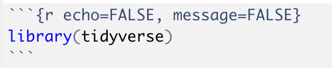
First, we need to load tidyverse.
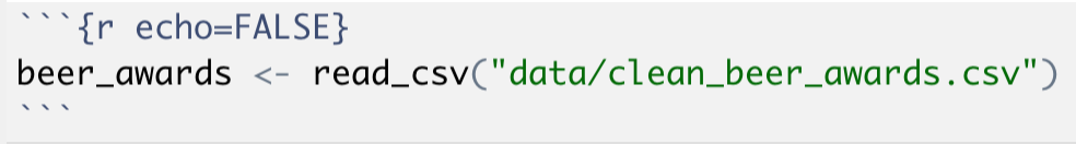
Then we can read data in.
## Parsed with column specification:
## cols(
##   medal = col_character(),
##   beer_name = col_character(),
##   brewery = col_character(),
##   city = col_character(),
##   state = col_character(),
##   category = col_character(),
##   year = col_double(),
##   macro_category = col_character(),
##   state_area = col_double(),
##   region = col_character(),
##   state_name = col_character(),
##   state_division = col_character()
## )
14.6 Data Tables
Use the function kable() to print out nice tables.
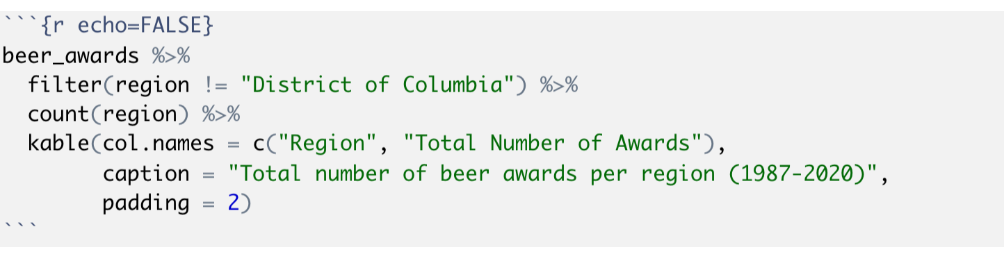
| Region | Total Number of Awards |
|---|---|
| North Central | 983 |
| Northeast | 537 |
| South | 787 |
| West | 2659 |
Whenever you have results with decimals, you can specify the number of digitis to display.
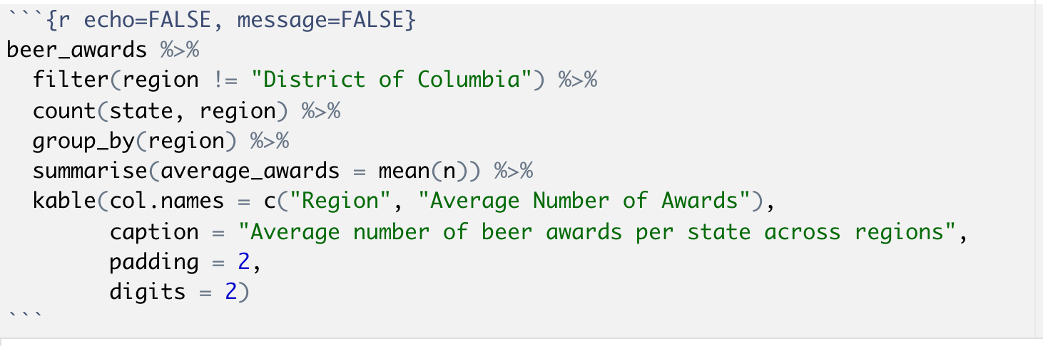
| Region | Average Number of Awards |
|---|---|
| North Central | 81.92 |
| Northeast | 59.67 |
| South | 52.47 |
| West | 204.54 |
14.7 Manual Tables
You might want to add an explanation table that does not come from your data. You can build tables manually in markdown by using the right dashes. Note that the default is left align. You can use : to change that alignment.
| Tables        | Are           | Cool  |
|---------------|:-------------:|------:|
| row 1 col 1   | row 1 col 2   | $1600 |
| row 2 col 1   | row 2 col 2   |   $12 |
| row 1 col 1 | row 3 col 2 | $1 || Tables | Are | Cool |
|---|---|---|
| row 1 col 1 | row 1 col 2 | $1600 |
| row 2 col 1 | row 2 col 2 | $12 |
| row 1 col 1 | row 3 col 2 | $1 |
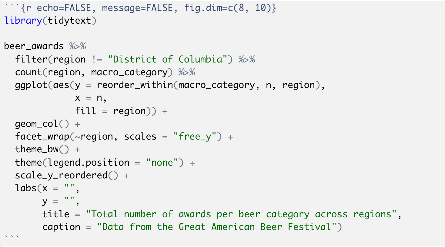
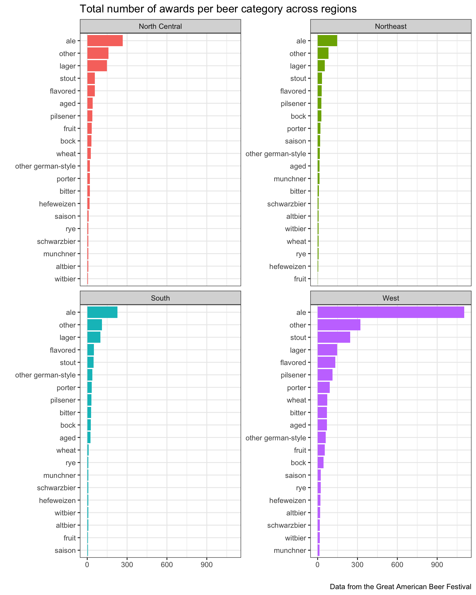
14.8 Plots
There are also a number of options that you can use for displaying plots nicely.
14.9 Knitting PDFs
The easiest way to install TeX in your computer (if you don’t have TeX/LaTeX installed already) is through the tinytext package.
Now you can change html_document to pdf_document to output a pdf instead of a html file.
14.10 DATA CHALLENGE 08
Accept data challenge 08 assignment