Module 11 Data Case Study 2
We’ve been working mainly with the tidyverse library, but today we will work with a few different libraries. The packages janitor and lubridate are very useful. Maybe sure you have these installed (use install.packages) before you load these libraries.
##
## Attaching package: 'janitor'
## The following objects are masked from 'package:stats':
##
## chisq.test, fisher.test11.1 Reading data from a URL
Today we are working with a large data set on global land temperatures. I added the csv file to github because it’s a very large file. You can use read_csv to read the file directly from github
global_temperatures <- read_csv("https://raw.githubusercontent.com/esoc214/fall2020_002_class_scripts/main/data/GlobalLandTemperaturesByCountry.csv") ## Parsed with column specification:
## cols(
## dt = col_date(format = ""),
## AverageTemperature = col_double(),
## AverageTemperatureUncertainty = col_double(),
## Country = col_character()
## )## Rows: 577,462
## Columns: 4
## $ dt <date> 1743-11-01, 1743-12-01, 1744-01-01, 174…
## $ AverageTemperature <dbl> 4.384, NA, NA, NA, NA, 1.530, 6.702, 11.…
## $ AverageTemperatureUncertainty <dbl> 2.294, NA, NA, NA, NA, 4.680, 1.789, 1.5…
## $ Country <chr> "Åland", "Åland", "Åland", "Åland", "Åla…11.2 Cleaning up column names
Column names from different data sets usually have a number of different casings (Camel, Pascal, Snake, Kebab Case, etc.). I like to use clean_names() to standardize column names to snake_case.
global_temperatures <- global_temperatures %>%
clean_names()
# inspect data
glimpse(global_temperatures)
## Rows: 577,462
## Columns: 4
## $ dt <date> 1743-11-01, 1743-12-01, 1744-01-01, 1…
## $ average_temperature <dbl> 4.384, NA, NA, NA, NA, 1.530, 6.702, 1…
## $ average_temperature_uncertainty <dbl> 2.294, NA, NA, NA, NA, 4.680, 1.789, 1…
## $ country <chr> "Åland", "Åland", "Åland", "Åland", "Å…11.3 Manipulating Dates
Now, let’s turn our attention to the dt column, which is a date.
## [1] "Date"There’s a number of functions we can run on a Date variable.
## [1] 1743 1743 1744 1744 1744 1744 1744 1744 1744 1744## [1] 11 12 1 2 3 4 5 6 7 8## [1] Nov Dec Jan Feb Mar Apr May Jun Jul Aug
## 12 Levels: Jan < Feb < Mar < Apr < May < Jun < Jul < Aug < Sep < ... < Dec## [1] 44 48 1 5 9 14 18 22 27 31We can create new columns in our data frame with year, month, and week extracted from dt in our data frame by using mutate.
## # A tibble: 577,462 x 7
##    dt         average_temperat… average_temperature_… country  year month decade
##    <date>                 <dbl>                 <dbl> <chr>   <dbl> <dbl>  <dbl>
##  1 1743-11-01              4.38                  2.29 Åland    1743    11   1740
##  2 1743-12-01             NA                    NA    Åland    1743    12   1740
##  3 1744-01-01             NA                    NA    Åland    1744     1   1740
##  4 1744-02-01             NA                    NA    Åland    1744     2   1740
##  5 1744-03-01             NA                    NA    Åland    1744     3   1740
##  6 1744-04-01              1.53                  4.68 Åland    1744     4   1740
##  7 1744-05-01              6.70                  1.79 Åland    1744     5   1740
##  8 1744-06-01             11.6                   1.58 Åland    1744     6   1740
##  9 1744-07-01             15.3                   1.41 Åland    1744     7   1740
## 10 1744-08-01             NA                    NA    Åland    1744     8   1740
## # … with 577,452 more rows
Instead of just printing to the console, let’s change the original data frame.
global_temperatures <- global_temperatures %>%
  mutate(year = year(dt),
         month = month(dt),
         decade = gsub("([12][0-9][0-9])[0-9]", "\\10", year))

# inspect changes
glimpse(global_temperatures)
## Rows: 577,462
## Columns: 7
## $ dt <date> 1743-11-01, 1743-12-01, 1744-01-01, 1…
## $ average_temperature <dbl> 4.384, NA, NA, NA, NA, 1.530, 6.702, 1…
## $ average_temperature_uncertainty <dbl> 2.294, NA, NA, NA, NA, 4.680, 1.789, 1…
## $ country <chr> "Åland", "Åland", "Åland", "Åland", "Å…
## $ year <dbl> 1743, 1743, 1744, 1744, 1744, 1744, 17…
## $ month <dbl> 11, 12, 1, 2, 3, 4, 5, 6, 7, 8, 9, 10,…
## $ decade <chr> "1740", "1740", "1740", "1740", "1740"…11.4 Extra Data libraries
If you need some hierarchical information that is not present in your data frame, such as continent based on country, check if there is a package that will do that for you. In our case, we will use the countrycode package.
Let’s look at our country variable.
## # A tibble: 243 x 2
##    country            n
##    <chr>          <int>
##  1 Afghanistan     2106
##  2 Africa          1965
##  3 Åland           3239
##  4 Albania         3239
##  5 Algeria         2721
##  6 American Samoa  1761
##  7 Andorra         3239
##  8 Angola          1878
##  9 Anguilla        2277
## 10 Antarctica       764
## # … with 233 more rows
We use the function countrycode() to get continent from a country name.
# create new column called continent
global_temperatures <- global_temperatures %>%
  mutate(continent = countrycode(sourcevar = country,
                            origin = "country.name",
                            destination = "continent"))
## Warning in countrycode(sourcevar = country, origin = "country.name", destination = "continent"): Some values were not matched unambiguously: Africa, Antarctica, Asia, Baker Island, Europe, French Southern And Antarctic Lands, Heard Island And Mcdonald Islands, Kingman Reef, North America, Oceania, Palmyra Atoll, Saint Martin, South America, South Georgia And The South Sandwich Isla, Virgin Islands## Rows: 577,462
## Columns: 8
## $ dt <date> 1743-11-01, 1743-12-01, 1744-01-01, 1…
## $ average_temperature <dbl> 4.384, NA, NA, NA, NA, 1.530, 6.702, 1…
## $ average_temperature_uncertainty <dbl> 2.294, NA, NA, NA, NA, 4.680, 1.789, 1…
## $ country <chr> "Åland", "Åland", "Åland", "Åland", "Å…
## $ year <dbl> 1743, 1743, 1744, 1744, 1744, 1744, 17…
## $ month <dbl> 11, 12, 1, 2, 3, 4, 5, 6, 7, 8, 9, 10,…
## $ decade <chr> "1740", "1740", "1740", "1740", "1740"…
## $ continent <chr> "Europe", "Europe", "Europe", "Europe"…Always check your data. Let’s look at continent more closely, especially since we got a warning message.
# why some continents were not assigned
global_temperatures %>%
  filter(is.na(continent)) %>%
  distinct(country)
## # A tibble: 15 x 1
## country
## <chr>
## 1 Africa
## 2 Antarctica
## 3 Asia
## 4 Baker Island
## 5 Europe
## 6 French Southern And Antarctic Lands
## 7 Heard Island And Mcdonald Islands
## 8 Kingman Reef
## 9 North America
## 10 Oceania
## 11 Palmyra Atoll
## 12 Saint Martin
## 13 South America
## 14 South Georgia And The South Sandwich Isla
## 15 Virgin IslandsIt seems we can eliminate the rows with NA for continent.
11.5 Exploring Data
Now that our data is clean and transformed, what’s our data question? The data frame is still very large, so some summarization would be helpful.
global_temp_continents  %>%
  group_by(decade, continent) %>%
  summarise(mean_temp = mean(average_temperature, na.rm = TRUE))
## `summarise()` has grouped output by 'decade'. You can override using the `.groups` argument.## # A tibble: 128 x 3
## # Groups: decade [28]
## decade continent mean_temp
## <chr> <chr> <dbl>
## 1 1740 Americas 2.62
## 2 1740 Europe 6.98
## 3 1750 Africa 19.8
## 4 1750 Americas 7.30
## 5 1750 Europe 8.53
## 6 1760 Africa 19.8
## 7 1760 Americas 6.44
## 8 1760 Europe 8.31
## 9 1770 Africa 20.1
## 10 1770 Americas 6.61
## # … with 118 more rowsIt’s still a long data frame, plotting helps here.
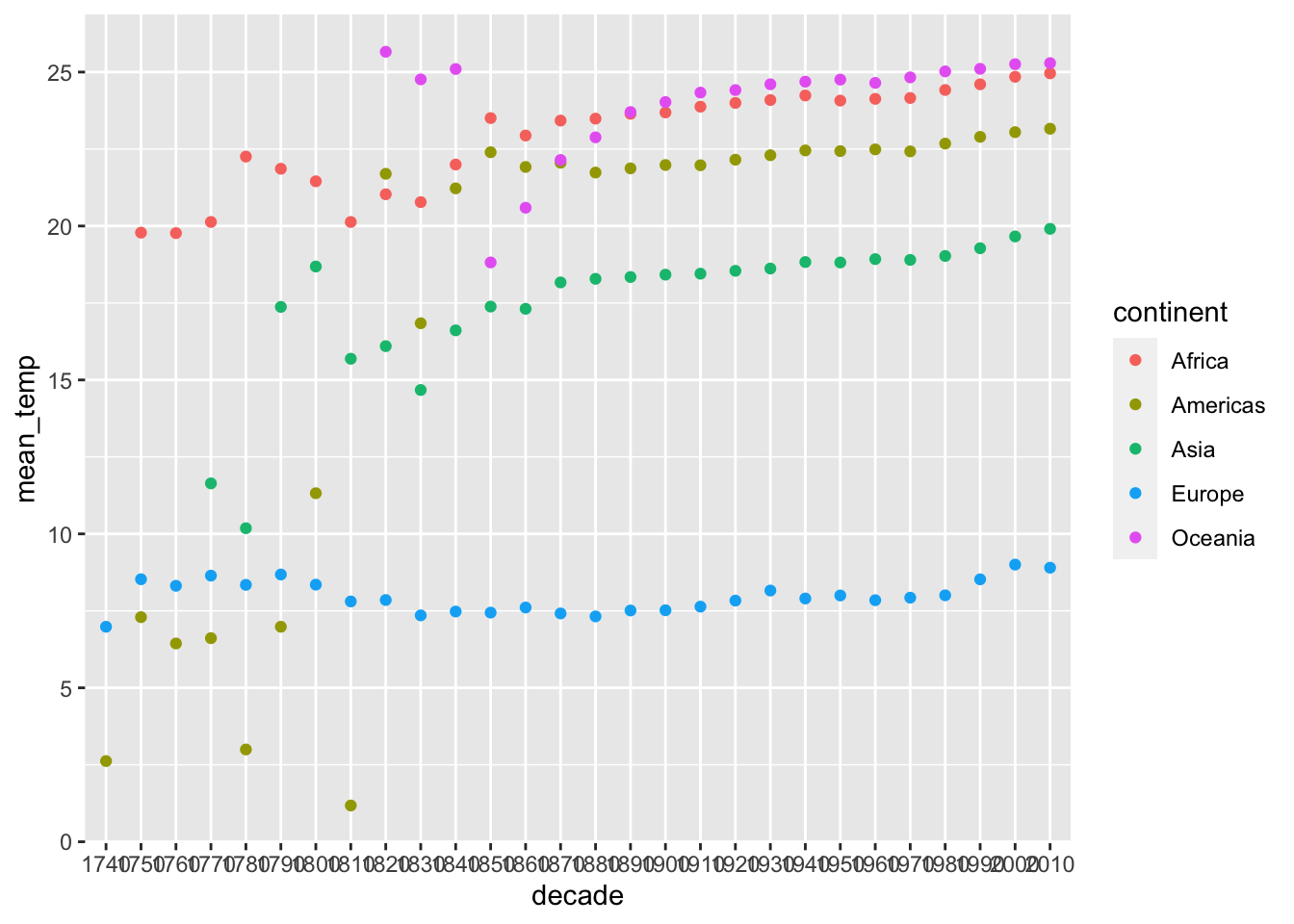
global_temp_continents  %>%
  group_by(decade, continent) %>%
  summarise(mean_temp = mean(average_temperature, na.rm = TRUE)) %>%
  ggplot(aes(x = decade, y = mean_temp, color = continent)) +
  geom_point()
## `summarise()` has grouped output by 'decade'. You can override using the `.groups` argument.
Looking at the plot above, how reliable do you think these temperatures are? Why?
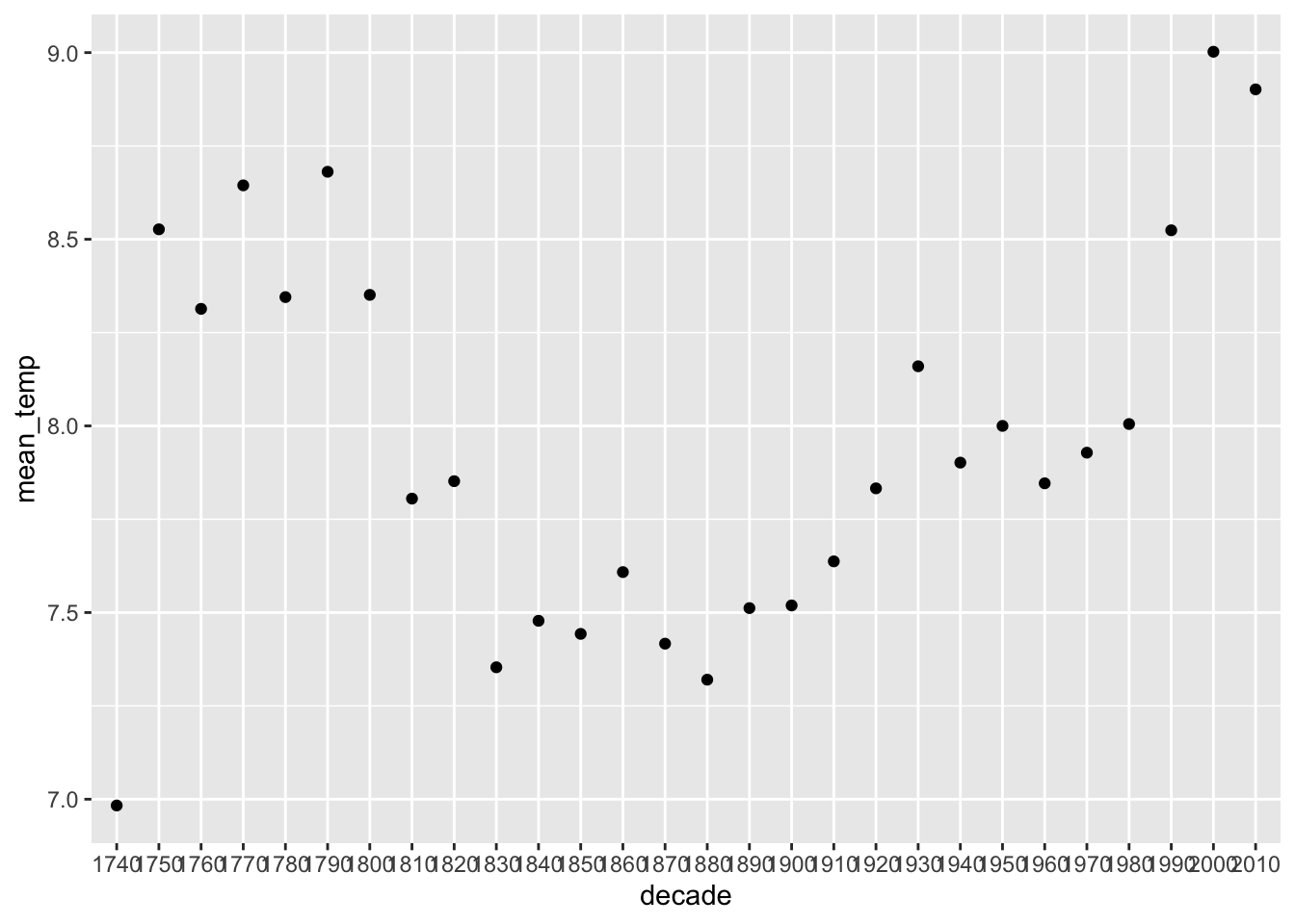
Let’s look at Europe only.
europe_temps  %>%
  group_by(decade) %>%
  summarise(mean_temp = mean(average_temperature, na.rm = TRUE)) %>%
  ggplot(aes(x = decade, y = mean_temp)) +
  geom_point()
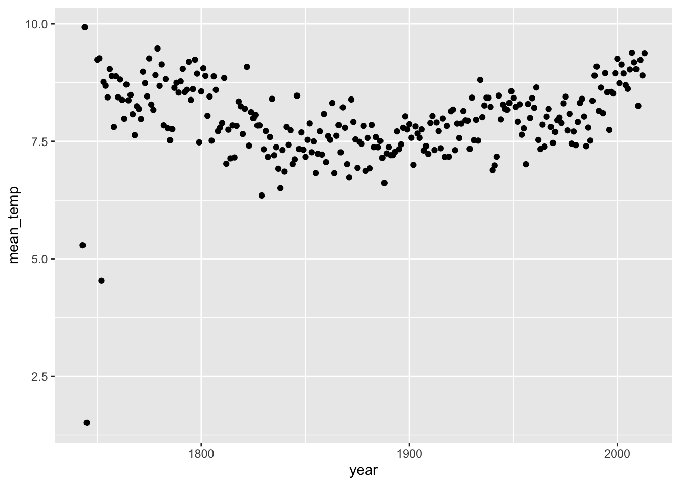
Now that we have filtered by continent, we can look at year instead of decade, because you have less information to plot (just one continent).
europe_temps  %>%
  group_by(year) %>%
  summarise(mean_temp = mean(average_temperature, na.rm = TRUE)) %>%
  ggplot(aes(x = year, y = mean_temp)) +
  geom_point()
## Warning: Removed 4 rows containing missing values (geom_point).
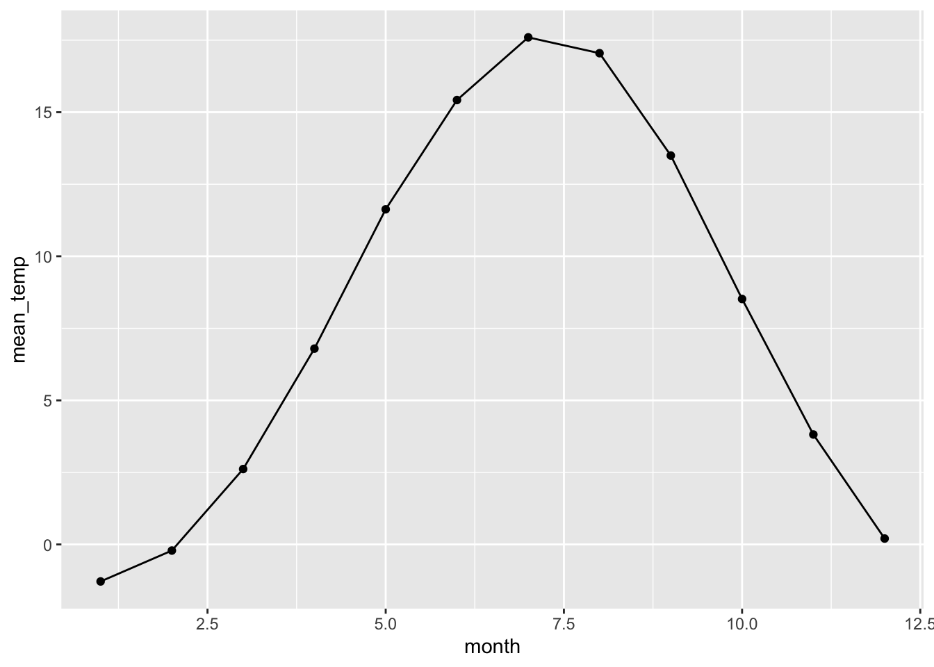
Let’s look at monthly temperatures
europe_temps  %>%
  group_by(month) %>%
  summarise(mean_temp = mean(average_temperature, na.rm = TRUE)) %>%
  ggplot(aes(x = month, y = mean_temp)) +
  geom_point() +
  geom_line()
Would this pattern, of temperature increase around June, be the same no matter the continent?
11.6 DATA CHALLENGE 06
Accept data challenge 06 assignment