Module 10 Data Case Study 1
This is our first case study of the semester. The goal of each case study is to consolidate the content we’ve covered so far in class, which at this point includes:
Load libraries using
library()Read data using
read_csv()orread_excel()Inspect data using
summary()orglimpse()and/orView()Review your data question (what variables do you need to answer your question?)
Explore data using the following functions:
count()group_by()+summarise()
- Plot data using the functions above and:
filter()mutate()gglot(aes())+geom_...
# load library
library(tidyverse)

# read data in
olympic_events <- read_csv("data/olympic_history_athlete_events.csv")
## Parsed with column specification:
## cols(
## ID = col_double(),
## Name = col_character(),
## Sex = col_character(),
## Age = col_double(),
## Height = col_double(),
## Weight = col_double(),
## Team = col_character(),
## NOC = col_character(),
## Games = col_character(),
## Year = col_double(),
## Season = col_character(),
## City = col_character(),
## Sport = col_character(),
## Event = col_character(),
## Medal = col_character()
## )## Parsed with column specification:
## cols(
## NOC = col_character(),
## region = col_character(),
## notes = col_character()
## )## Rows: 271,116
## Columns: 15
## $ ID <dbl> 1, 2, 3, 4, 5, 5, 5, 5, 5, 5, 6, 6, 6, 6, 6, 6, 6, 6, 7, 7, 7,…
## $ Name <chr> "A Dijiang", "A Lamusi", "Gunnar Nielsen Aaby", "Edgar Lindena…
## $ Sex <chr> "M", "M", "M", "M", "F", "F", "F", "F", "F", "F", "M", "M", "M…
## $ Age <dbl> 24, 23, 24, 34, 21, 21, 25, 25, 27, 27, 31, 31, 31, 31, 33, 33…
## $ Height <dbl> 180, 170, NA, NA, 185, 185, 185, 185, 185, 185, 188, 188, 188,…
## $ Weight <dbl> 80, 60, NA, NA, 82, 82, 82, 82, 82, 82, 75, 75, 75, 75, 75, 75…
## $ Team <chr> "China", "China", "Denmark", "Denmark/Sweden", "Netherlands", …
## $ NOC <chr> "CHN", "CHN", "DEN", "DEN", "NED", "NED", "NED", "NED", "NED",…
## $ Games <chr> "1992 Summer", "2012 Summer", "1920 Summer", "1900 Summer", "1…
## $ Year <dbl> 1992, 2012, 1920, 1900, 1988, 1988, 1992, 1992, 1994, 1994, 19…
## $ Season <chr> "Summer", "Summer", "Summer", "Summer", "Winter", "Winter", "W…
## $ City <chr> "Barcelona", "London", "Antwerpen", "Paris", "Calgary", "Calga…
## $ Sport <chr> "Basketball", "Judo", "Football", "Tug-Of-War", "Speed Skating…
## $ Event <chr> "Basketball Men's Basketball", "Judo Men's Extra-Lightweight",…
## $ Medal <chr> NA, NA, NA, "Gold", NA, NA, NA, NA, NA, NA, NA, NA, NA, NA, NA…## Rows: 230
## Columns: 3
## $ NOC <chr> "AFG", "AHO", "ALB", "ALG", "AND", "ANG", "ANT", "ANZ", "ARG",…
## $ region <chr> "Afghanistan", "Curacao", "Albania", "Algeria", "Andorra", "An…
## $ notes <chr> NA, "Netherlands Antilles", NA, NA, NA, NA, "Antigua and Barbu…10.1 Data Questions
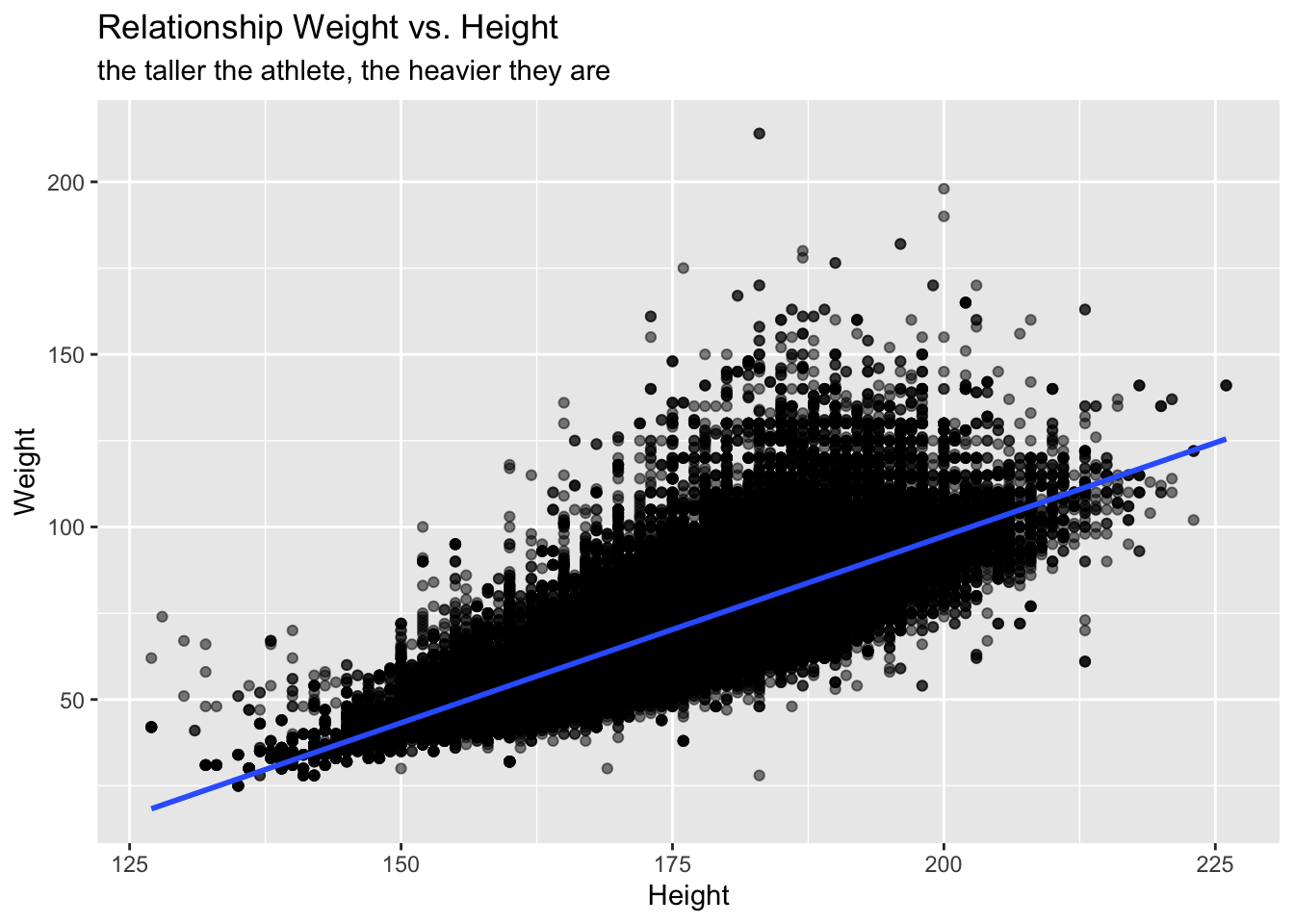
Has athlete height and weight changed over time overall?
Has height and weight changed over time for the top 5 countries with the most medals?
10.2 Data Exploration
Suggestions of data exploration:
What type of olympics? What years? How many athletes per game?
## # A tibble: 51 x 2
##    Games           n
##    <chr>       <int>
##  1 1896 Summer   380
##  2 1900 Summer  1936
##  3 1904 Summer  1301
##  4 1906 Summer  1733
##  5 1908 Summer  3101
##  6 1912 Summer  4040
##  7 1920 Summer  4292
##  8 1924 Summer  5233
##  9 1924 Winter   460
## 10 1928 Summer  4992
## # … with 41 more rows
This data set is huge, the plot below will take a while to process:
What are the top countries for medal count?
## # A tibble: 783 x 3
##    Team          Medal      n
##    <chr>         <chr>  <int>
##  1 United States Gold    2474
##  2 United States Silver  1512
##  3 United States Bronze  1233
##  4 Soviet Union  Gold    1058
##  5 Soviet Union  Silver   716
##  6 Germany       Gold     679
##  7 Germany       Bronze   678
##  8 Soviet Union  Bronze   677
##  9 Germany       Silver   627
## 10 Great Britain Silver   582
## # … with 773 more rows
10.3 Calculate height and weight relationship
It’s difficult to plot three numeric variables (in this case we want to plot weight, height, across different years) with so many data points. So I’ll create a new variable in my data frame with is the relationship between height and weight (i.e., kg per cm).
## # A tibble: 271,116 x 3
## Weight Height kg_per_cm
## <dbl> <dbl> <dbl>
## 1 80 180 0.444
## 2 60 170 0.353
## 3 NA NA NA
## 4 NA NA NA
## 5 82 185 0.443
## 6 82 185 0.443
## 7 82 185 0.443
## 8 82 185 0.443
## 9 82 185 0.443
## 10 82 185 0.443
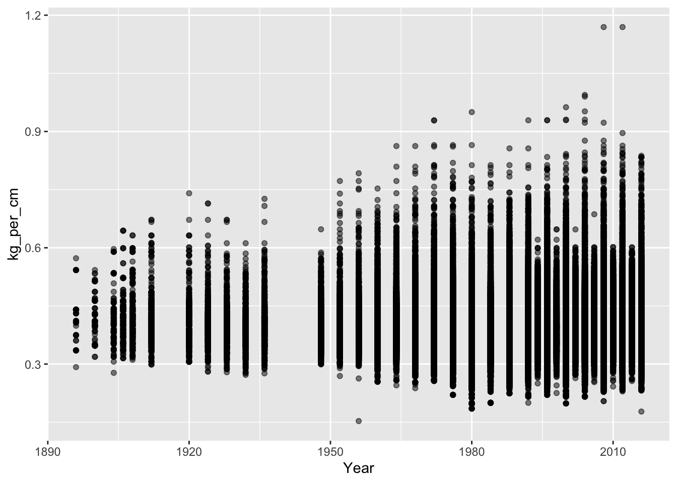
## # … with 271,106 more rows10.4 Plot kilos per centimeter across years
Now that we have this new variable, which is kilos per centimeters, we can plot this variable across years.
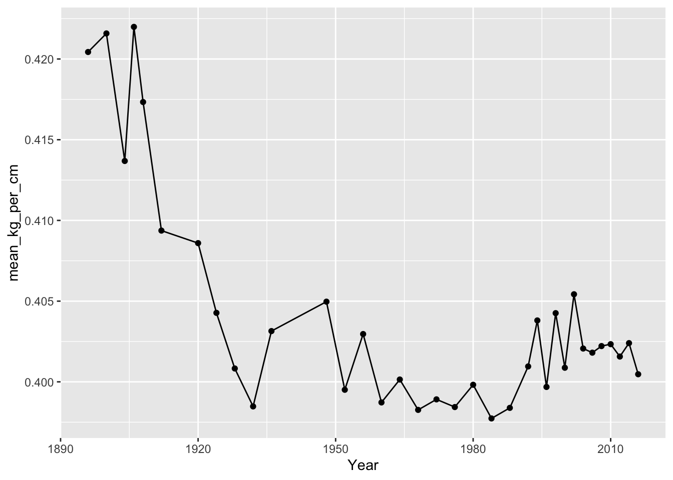
Let’s see if summarised data (i.e., mean of kg_per_cm across year), makes more sense.
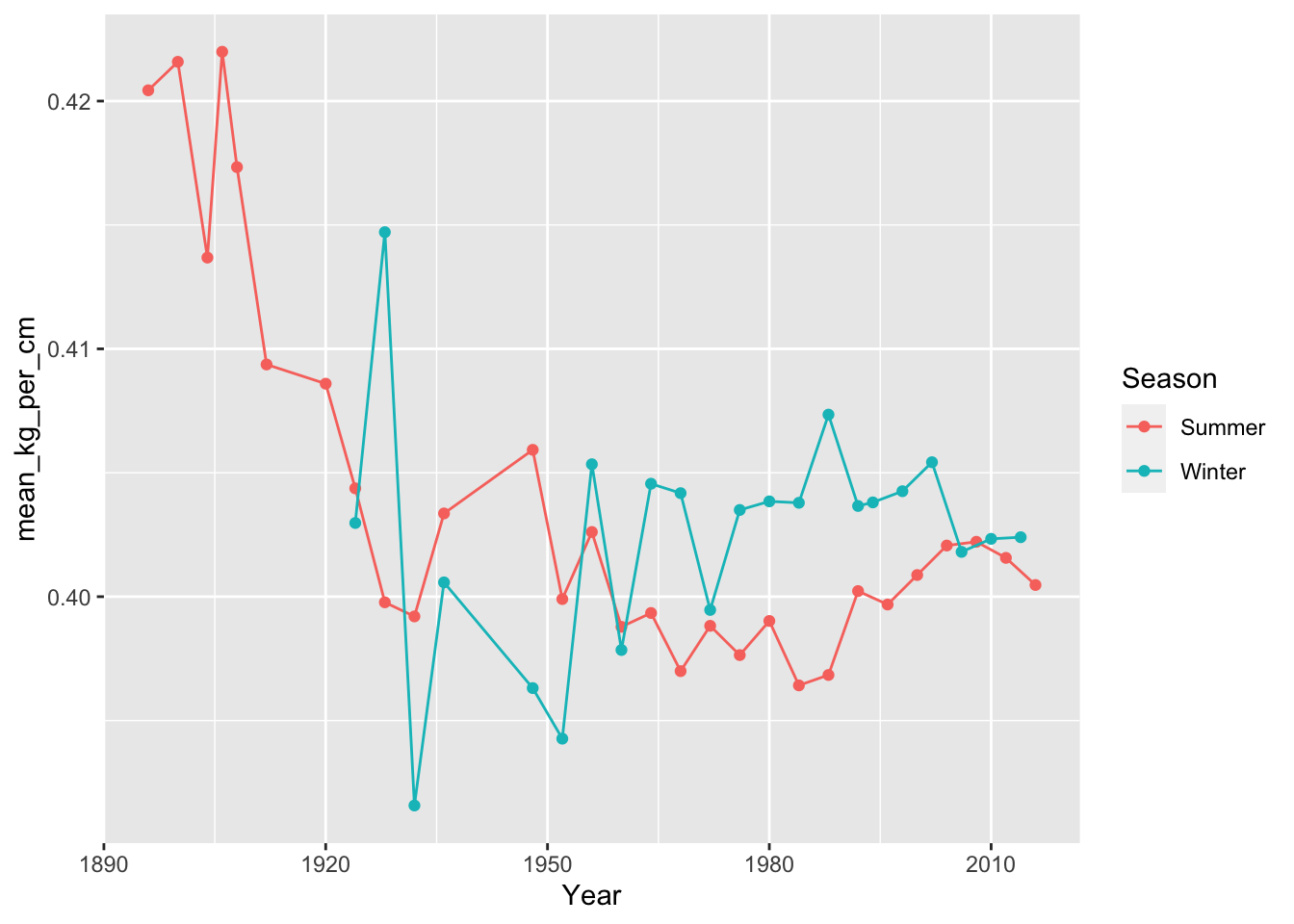
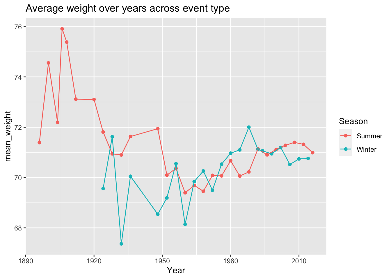
Let’s split by Summer vs. Winter olympics.
10.5 Plot weight over time
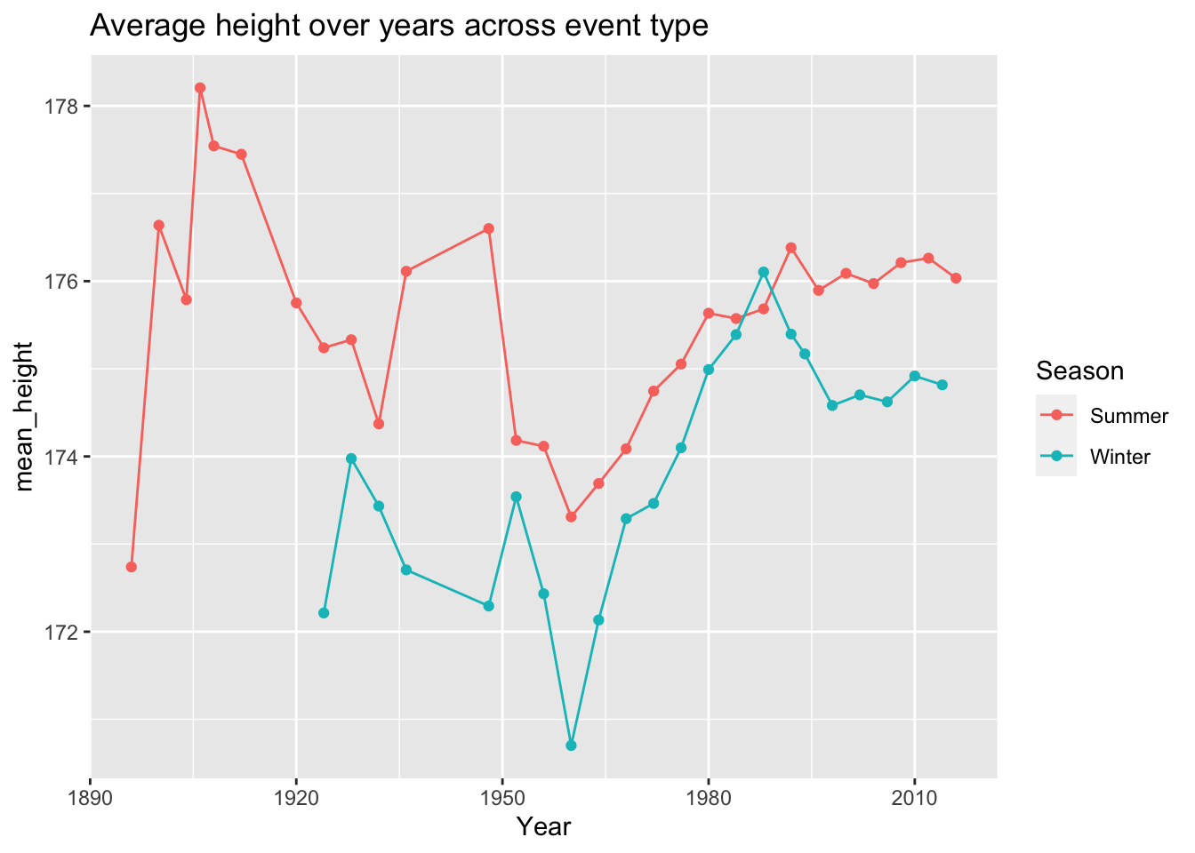
10.6 Plot height over time
10.7 Data Filtering
Get only top 5 countries for highest medal count
## # A tibble: 5 x 2
##   Team              n
##   <chr>         <int>
## 1 United States  5219
## 2 Soviet Union   2451
## 3 Germany        1984
## 4 Great Britain  1673
## 5 France         1550
Create a list of these countries to filter the largest data set to create a smaller data frame.
## Rows: 56,100
## Columns: 16
## $ ID <dbl> 6, 6, 6, 6, 6, 6, 6, 6, 7, 7, 7, 7, 7, 7, 7, 7, 34, 52, 56,…
## $ Name <chr> "Per Knut Aaland", "Per Knut Aaland", "Per Knut Aaland", "P…
## $ Sex <chr> "M", "M", "M", "M", "M", "M", "M", "M", "M", "M", "M", "M",…
## $ Age <dbl> 31, 31, 31, 31, 33, 33, 33, 33, 31, 31, 31, 31, 33, 33, 33,…
## $ Height <dbl> 188, 188, 188, 188, 188, 188, 188, 188, 183, 183, 183, 183,…
## $ Weight <dbl> 75, 75, 75, 75, 75, 75, 75, 75, 72, 72, 72, 72, 72, 72, 72,…
## $ Team <chr> "United States", "United States", "United States", "United …
## $ NOC <chr> "USA", "USA", "USA", "USA", "USA", "USA", "USA", "USA", "US…
## $ Games <chr> "1992 Winter", "1992 Winter", "1992 Winter", "1992 Winter",…
## $ Year <dbl> 1992, 1992, 1992, 1992, 1994, 1994, 1994, 1994, 1992, 1992,…
## $ Season <chr> "Winter", "Winter", "Winter", "Winter", "Winter", "Winter",…
## $ City <chr> "Albertville", "Albertville", "Albertville", "Albertville",…
## $ Sport <chr> "Cross Country Skiing", "Cross Country Skiing", "Cross Coun…
## $ Event <chr> "Cross Country Skiing Men's 10 kilometres", "Cross Country …
## $ Medal <chr> NA, NA, NA, NA, NA, NA, NA, NA, NA, NA, NA, NA, NA, NA, NA,…
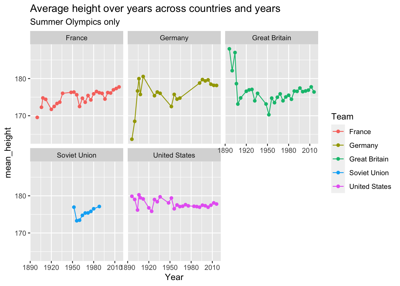
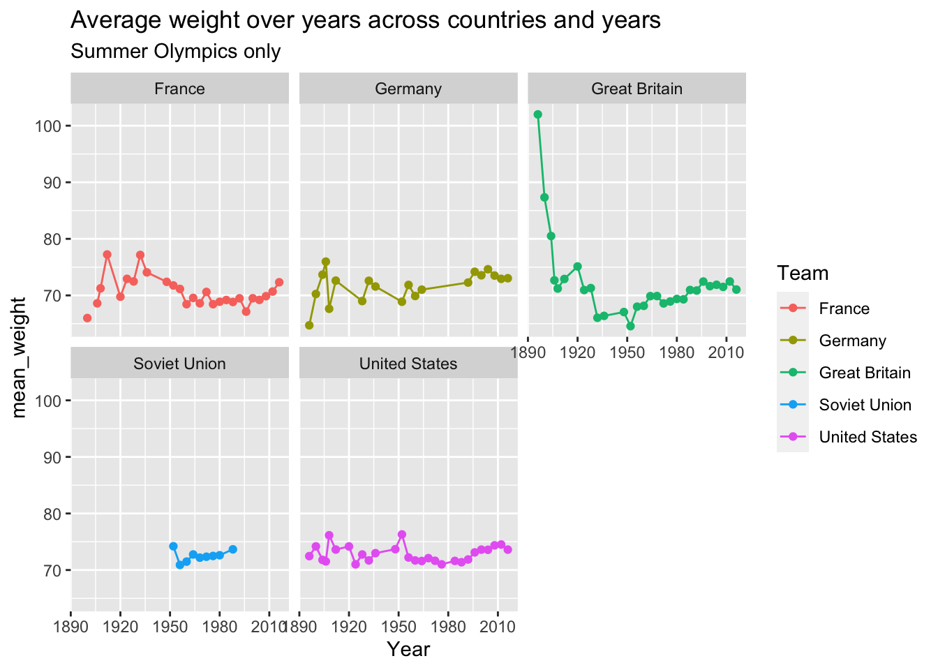
## $ kg_per_cm <dbl> 0.3989362, 0.3989362, 0.3989362, 0.3989362, 0.3989362, 0.39…10.8 Plot height and weight across countries over the years
10.9 Solving the problem of team name changes over time
We can use name of Olympic committee (NOC) to standardized Team to country
## # A tibble: 1,231 x 3
##    NOC   Team                     n
##    <chr> <chr>                <int>
##  1 AFG   Afghanistan            126
##  2 AHO   Netherlands Antilles    79
##  3 ALB   Albania                 70
##  4 ALG   Algeria                551
##  5 AND   Andorra                169
##  6 ANG   Angola                 267
##  7 ANT   Antigua and Barbuda    133
##  8 ANZ   Australasia             77
##  9 ANZ   Sydney Rowing Club       9
## 10 ARG   Acturus                  2
## # … with 1,221 more rows
The olympic_noc_regions data frame can help with that process.
## # A tibble: 6 x 3
##   NOC   region      notes
##   <chr> <chr>       <chr>
## 1 AFG   Afghanistan <NA>
## 2 AHO   Curacao     Netherlands Antilles
## 3 ALB   Albania     <NA>
## 4 ALG   Algeria     <NA>
## 5 AND   Andorra     <NA>
## 6 ANG   Angola      <NA>
We can add region to our olympic_events data frame by joining the olympic_events data frame with the olympic_noc_regions data frame by the NOC column. For that we will use the left_join() function.
## Joining, by = "NOC"## # A tibble: 230 x 3
## NOC region n
## <chr> <chr> <int>
## 1 AFG Afghanistan 126
## 2 AHO Curacao 79
## 3 ALB Albania 70
## 4 ALG Algeria 551
## 5 AND Andorra 169
## 6 ANG Angola 267
## 7 ANT Antigua 133
## 8 ANZ Australia 86
## 9 ARG Argentina 3297
## 10 ARM Armenia 221
## # … with 220 more rowsLet’s check what we have for Russia now.
## # A tibble: 3 x 3
##   NOC   region     n
##   <chr> <chr>  <int>
## 1 EUN   Russia   864
## 2 RUS   Russia  5143
## 3 URS   Russia  5685
We can now calculate medals per region instead of team name. Get only top 5 countries for highest medal count
## # A tibble: 5 x 2
##   region      n
##   <chr>   <int>
## 1 USA      5637
## 2 Russia   3947
## 3 Germany  3756
## 4 UK       2068
## 5 France   1777
10.10 DATA CHALLENGE 05
Accept data challenge 05 assignment