Reproducing Open Science Research 1

This tutorial took place on September 1, 2023. Here’s the session recording.

Data

For this tutorial, we will be reproduction the data analysis at an Open Science repository. We are going to be using data from the IRIS database.

Here’s an excerpt of the study’s abstract:

This study investigated the effects of task complexity on child learners’ second language (L2) gains, the relationship between aptitude and L2 development, and the extent to which task complexity influences this relationship when recasts are provided. Sixty child EFL learners were assigned to two experimental groups. During the treatment, one group completed simple information transmission tasks, whereas the other group performed complex decision-making tasks. In response to errors in the use of the present third person singular verb forms, participants received recasts. L2 development was measured through oral production, written production, and elicited imitation tests. Aptitude was assessed through LLAMA D, LLAMA E, and LLAMA F.

Our first step it to load the tidyverse library (RStudio will prompt you to install it).

# load library for data analysis
library(tidyverse)

Download the data and add it to your project inside a folder called data.

Now we read the data in:

# read data in
child_l2_data <- read_csv("data/Data_Kourtali_Revesz.csv")

It’s always a good idea to inspect the data to make sure everything looks good.

glimpse(child_l2_data)

Rows: 60
Columns: 61
$ Participant                   <dbl> 1, 3, 11, 12, 15, 25, 26, 32, 40, 41, 43…
$ Time                          <dbl> 1, 1, 1, 1, 1, 1, 1, 1, 1, 1, 1, 1, 1, 1…
$ Group                         <dbl> 1, 1, 1, 1, 1, 1, 1, 1, 1, 1, 1, 1, 1, 1…
$ Duration_English              <dbl> 6.0, 5.0, 4.0, 5.0, 4.0, 4.0, 6.0, 7.0, …
$ Listening                     <dbl> 6, 10, 5, 5, 3, 5, 7, 10, 6, 9, 10, 7, 9…
$ Oral_Production_Pre           <dbl> 26.31, 18.75, 0.00, 0.00, 0.00, 0.00, 0.…
$ Written_Production_Pre        <dbl> 0.00, 9.09, 0.00, 0.00, 0.00, 0.00, 8.33…
$ Oral_Production_Post          <dbl> 26.66, 28.57, 0.00, 0.00, 0.00, 53.33, 3…
$ Written_Production_Post       <dbl> 61.53, 75.00, 0.00, 58.33, 0.00, 100.00,…
$ EI                            <dbl> 29.16, 29.10, 0.00, 12.50, 0.00, 4.16, 4…
$ EI_GRAM                       <dbl> 41.66, 50.00, 0.00, 25.00, 0.00, 8.33, 8…
$ EI_UNGRAM                     <dbl> 16.66, 8.33, 0.00, 0.00, 0.00, 0.00, 0.0…
$ LLAMA_D                       <dbl> 45, 10, 20, 15, 30, 25, 25, 35, 35, 35, …
$ LLAMA_E                       <dbl> 50, 0, 0, 40, 60, 0, 40, 90, 10, 30, 70,…
$ LLAMA_F                       <dbl> 0, 40, 20, 10, 0, 40, 50, 10, 30, 20, 0,…
$ Recasts_T1                    <dbl> 11, 10, 12, 16, 15, 3, 8, 9, 9, 12, 6, 9…
$ SU_T1_Number                  <dbl> 7, 8, 0, 0, 1, 1, 0, 7, 3, 3, 3, 1, 0, 6…
$ SU_T1_Percentage              <dbl> 63.63, 80.00, 0.00, 0.00, 6.66, 33.33, 0…
$ OC_T1_OVERALL                 <dbl> 19, 15, 13, 22, 15, 13, 15, 25, 13, 12, …
$ OC_T1                         <dbl> 18, 15, 13, 19, 15, 13, 15, 25, 13, 12, …
$ Recasts_T1_Percentage         <dbl> 61.11, 66.66, 92.30, 84.21, 100.00, 23.0…
$ CP_T1_Number                  <dbl> 6, 5, 1, 0, 0, 10, 7, 16, 4, 0, 7, 5, 9,…
$ CP_T1_Percentage              <dbl> 31.57, 33.33, 7.69, 0.00, 0.00, 76.92, 4…
$ Recasts_T2                    <dbl> 4, 9, 12, 10, 15, 3, 4, 1, 7, 8, 0, 6, 0…
$ SU_T2_Number                  <dbl> 4, 6, 2, 0, 0, 0, 0, 1, 7, 0, 0, 0, 0, 3…
$ SU_T2_Percentage              <dbl> 100.00, 66.66, 16.66, 0.00, 0.00, 0.00, …
$ OC_T2_OVERALL                 <dbl> 21, 14, 14, 19, 15, 14, 15, 22, 15, 14, …
$ OC_T2                         <dbl> 20, 14, 14, 18, 15, 14, 15, 22, 15, 14, …
$ Recasts_T2_percentage         <dbl> 20.00, 64.28, 85.71, 55.55, 100.00, 21.4…
$ CP_T2_Number                  <dbl> 15, 5, 2, 7, 0, 11, 11, 21, 8, 6, 13, 10…
$ CP_T2_Percentage              <dbl> 71.42, 35.71, 14.28, 36.84, 0.00, 78.57,…
$ ME_1                          <dbl> 2, 2, 5, 3, 2, 2, 1, 3, 6, 2, 3, 5, 5, 8…
$ ME_2                          <dbl> 2, 2, 5, 3, 3, 3, 1, 2, 2, 2, 2, 2, 5, 8…
$ Overall_Dif_T1                <dbl> 1, 2, 5, 3, 6, 1, 1, 1, 4, 1, 3, 1, 5, 1…
$ Overall_Dif_T2                <dbl> 1, 2, 4, 2, 6, 3, 1, 2, 4, 1, 2, 1, 4, 1…
$ Ling_Dif_T1                   <dbl> 1, 2, 6, 2, 3, 2, 1, 2, 4, 3, 2, 2, 4, 1…
$ Ling_Dif_T2                   <dbl> 1, 2, 6, 3, 4, 2, 1, 2, 3, 3, 2, 1, 4, 1…
$ Perceiv_Perf_T1               <dbl> 2, 3, 5, 3, 8, 7, 1, 4, 5, 2, 3, 3, 5, 2…
$ Perceiv_Perf_T2               <dbl> 1, 3, 5, 3, 7, 6, 1, 3, 5, 3, 2, 2, 5, 1…
$ Recasts_Number_total          <dbl> 15, 19, 24, 26, 30, 6, 12, 10, 16, 20, 6…
$ SU_Number_total               <dbl> 11, 14, 2, 0, 1, 1, 0, 8, 10, 3, 3, 1, 0…
$ SU_Percentage_total           <dbl> 73.33, 73.68, 8.33, 0.00, 3.33, 16.67, 0…
$ OC_TOTAL                      <dbl> 38, 29, 27, 37, 30, 27, 30, 47, 28, 26, …
$ Elicited_Imitation_Total_Pre  <dbl> 7, 7, 0, 3, 0, 1, 1, 4, 3, 4, 11, 5, 3, …
$ Elicited_Imitation_Gr_Pre     <dbl> 5, 6, 0, 3, 0, 1, 1, 3, 1, 3, 11, 5, 3, …
$ Elicited_Imitation_Ungr_Pre   <dbl> 2, 1, 0, 0, 0, 0, 0, 1, 2, 1, 0, 0, 0, 5…
$ Elicited_Imitation_Total_Post <dbl> 5, 10, 0, 8, 1, 0, 3, 17, 9, 7, 11, 14, …
$ Elicited_Imitation_Gr_Post    <dbl> 4, 10, 0, 6, 1, 0, 2, 9, 5, 7, 10, 10, 6…
$ Elicited_Imitation_Ungr_Post  <dbl> 1, 0, 0, 2, 0, 0, 1, 8, 4, 0, 1, 4, 0, 1…
$ Gain_oral                     <dbl> 0.35, 9.82, 0.00, 0.00, 0.00, 53.33, 30.…
$ Gain_written                  <dbl> 61.53, 65.91, 0.00, 58.33, 0.00, 100.00,…
$ Gain_EI                       <dbl> -2, 3, 0, 5, 1, -1, 2, 13, 6, 3, 0, 9, 3…
$ Gain_EI_Gr                    <dbl> -1, 4, 0, 3, 1, -1, 1, 6, 4, 4, -1, 5, 3…
$ Gain_EI_Ungr                  <dbl> -1, -1, 0, 2, 0, 0, 1, 7, 2, -1, 1, 4, 0…
$ CP_both_tasks                 <dbl> 21, 10, 3, 7, 0, 21, 18, 37, 12, 6, 20, …
$ ZRE_1                         <dbl> 2.94, 1.95, -0.53, -0.53, -0.53, -0.53, …
$ ZRE_2                         <dbl> -0.24, -0.18, -1.17, -1.17, -1.17, 0.69,…
$ OralProPre_log                <dbl> 3.27, 2.93, 0.00, 0.00, 0.00, 0.00, 0.00…
$ OralProPost_log               <dbl> 3.28, 3.35, 0.00, 0.00, 0.00, 3.98, 3.43…
$ ZRE_3                         <dbl> 2.22, 1.93, -0.58, -0.58, -0.58, -0.58, …
$ ZRE_4                         <dbl> 0.42, 0.46, -1.39, -1.39, -1.39, 0.81, 0…

Participants (page 187)

The final pool of participants included 26 females and 34 males

There should be 60 participants in the data.

The study employed a pretest–posttest design with two treatment sessions. Par- ticipants were assigned to one of two experimental groups through stratified random sampling, taking into account their pretest, proficiency, aptitude test results, and length of prior English study.

child_l2_data %>% 
  count(Group)

Group	n
1	30
2	30

A series of independent-samples t-tests targeting the variables length of previous English study, and performance on the proficiency test confirmed that the two groups were comparable.

group_1_data <- child_l2_data %>%
  filter(Group == 1)

group_2_data <- child_l2_data %>%
  filter(Group == 2)

English study,t=0.33,p=.75,d=0.08

t.test(group_1_data$Duration_English, 
       group_2_data$Duration_English)

    Welch Two Sample t-test

data:  group_1_data$Duration_English and group_2_data$Duration_English
t = 0.32672, df = 56.749, p-value = 0.7451
alternative hypothesis: true difference in means is not equal to 0
95 percent confidence interval:
 -0.5129511  0.7129511
sample estimates:
mean of x mean of y 
      4.7       4.6 

proficiency,t=0.07,p=.95,d=0.01

t.test(group_1_data$Listening, 
       group_2_data$Listening)

    Welch Two Sample t-test

data:  group_1_data$Listening and group_2_data$Listening
t = 0.061574, df = 57.922, p-value = 0.9511
alternative hypothesis: true difference in means is not equal to 0
95 percent confidence interval:
 -1.050337  1.117004
sample estimates:
mean of x mean of y 
 5.833333  5.800000 

T-test Effect Size using Cohen’s d Measure https://www.datanovia.com/en/lessons/t-test-effect-size-using-cohens-d-measure/

library(rstatix)
child_l2_data %>%
  cohens_d(Duration_English ~ Group)

.y.	group1	group2	effsize	n1	n2	magnitude
Duration_English	1	2	0.0843597	30	30	negligible

child_l2_data %>%
  cohens_d(Listening ~ Group)

.y.	group1	group2	effsize	n1	n2	magnitude
Listening	1	2	0.0158983	30	30	negligible

Statistical Analyses (page 196)

Table 1 Descriptive statistics for the perceived mental effort scale

The standard error is calculated by dividing the standard deviation by the sample size’s square root. The standard error is most useful as a means of calculating a confidence interval. For a large sample, a 95% confidence interval is obtained as the values 1.96×SE either side of the mean (https://www.ncbi.nlm.nih.gov/pmc/articles/PMC1255808).

child_l2_data %>%
  group_by(Group) %>%
  summarize(n = n(),
            mean_ME_1 = mean(ME_1),
            sd_ME_1 = sd(ME_1),
            mean_ME_2 = mean(ME_2),
            sd_ME_2 = sd(ME_2)) %>%
  mutate(lower_ci_ME_1 = mean_ME_1 - qt(1 - (.05 / 2), n - 1) * sd_ME_1/sqrt(n),
         upper_ci_ME_1 = mean_ME_1 + qt(1 - (.05 / 2), n - 1) * sd_ME_1/sqrt(n),
         lower_ci_ME_2 = mean_ME_2 - qt(1 - (.05 / 2), n - 1) * sd_ME_2/sqrt(n),
         upper_ci_ME_2 = mean_ME_2 + qt(1 - (.05 / 2), n - 1) * sd_ME_2/sqrt(n))

Group	n	mean_ME_1	sd_ME_1	mean_ME_2	sd_ME_2	lower_ci_ME_1	upper_ci_ME_1	lower_ci_ME_2	upper_ci_ME_2
1	30	3.833333	1.743626	3.433333	1.715715	3.182253	4.484414	2.792675	4.073992
2	30	5.933333	1.910648	5.233333	2.358891	5.219886	6.646781	4.352509	6.114158

Table 4 Results for the linear regression models examining the effects of task complexity on the oral and written production tests

The way it is in the paper: group is a numeric variable

model_1 <- lm(ME_1 ~ Group, child_l2_data)

library(effects)
effect("Group", model_1) %>%
  data.frame()

Group	fit	se	lower	upper
1.0	3.833333	0.3339362	3.164887	4.501779
1.2	4.253333	0.2753709	3.702119	4.804548
1.5	4.883333	0.2361286	4.410671	5.355996
1.8	5.513333	0.2753709	4.962119	6.064548
2.0	5.933333	0.3339362	5.264887	6.601779

# linear regression (recreation of table 4 on page 200)
model_table_4 <- child_l2_data %>%
  lm(formula = Oral_Production_Post ~ Oral_Production_Pre + Group)

summary(model_table_4)

Call:
lm(formula = Oral_Production_Post ~ Oral_Production_Pre + Group, 
    data = .)

Residuals:
    Min      1Q  Median      3Q     Max 
-41.942 -21.363  -4.573  21.869  66.482 

Coefficients:
                    Estimate Std. Error t value Pr(>|t|)    
(Intercept)          44.0133    11.1696   3.940 0.000224 ***
Oral_Production_Pre   1.3947     0.4662   2.991 0.004099 ** 
Group               -15.9727     6.9541  -2.297 0.025320 *  
---
Signif. codes:  0 '***' 0.001 '**' 0.01 '*' 0.05 '.' 0.1 ' ' 1

Residual standard error: 26.93 on 57 degrees of freedom
Multiple R-squared:  0.2022,    Adjusted R-squared:  0.1742 
F-statistic: 7.222 on 2 and 57 DF,  p-value: 0.001601

effect("Group", model_table_4) %>%
  data.frame() %>%
  ggplot(aes(x = Group,
             y = fit,
             ymin = lower,
             ymax = upper)) +
  geom_errorbar() +
  geom_label(aes(label = format(fit, digits = 2)))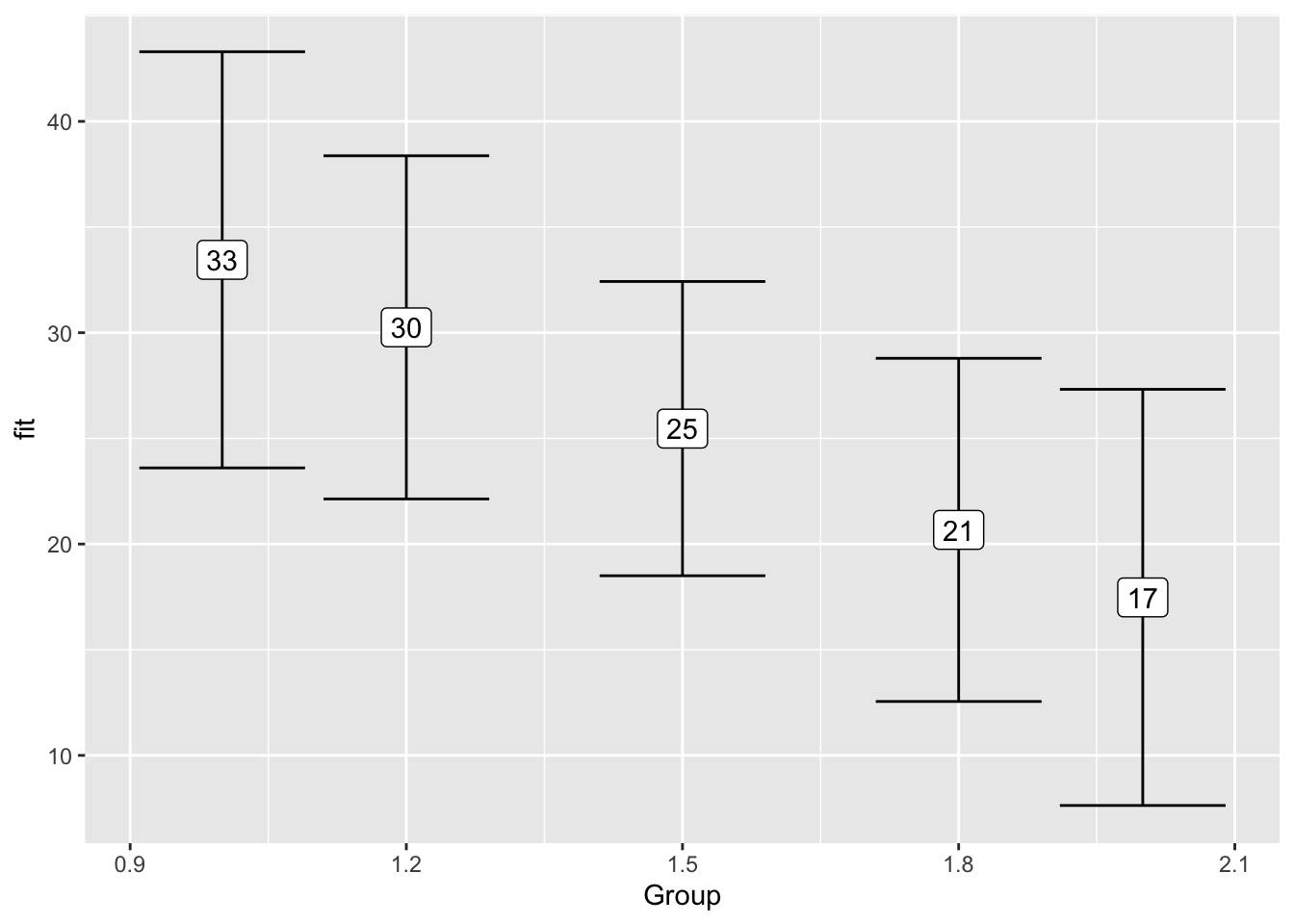

The correct way: group is a categorical (factor) variable

child_l2_data <- child_l2_data %>%
  mutate(group = factor(Group))

model_1 <- lm(ME_1 ~ group, child_l2_data)

effect("group", model_1) %>%
  data.frame()

group	fit	se	lower	upper
1	3.833333	0.3339362	3.164887	4.501779
2	5.933333	0.3339362	5.264887	6.601779

model_table_4 <- child_l2_data %>%
  lm(formula = Oral_Production_Post ~ Oral_Production_Pre + group)

summary(model_table_4)

Call:
lm(formula = Oral_Production_Post ~ Oral_Production_Pre + group, 
    data = .)

Residuals:
    Min      1Q  Median      3Q     Max 
-41.942 -21.363  -4.573  21.869  66.482 

Coefficients:
                    Estimate Std. Error t value Pr(>|t|)    
(Intercept)          28.0406     5.2577   5.333 1.72e-06 ***
Oral_Production_Pre   1.3947     0.4662   2.991   0.0041 ** 
group2              -15.9727     6.9541  -2.297   0.0253 *  
---
Signif. codes:  0 '***' 0.001 '**' 0.01 '*' 0.05 '.' 0.1 ' ' 1

Residual standard error: 26.93 on 57 degrees of freedom
Multiple R-squared:  0.2022,    Adjusted R-squared:  0.1742 
F-statistic: 7.222 on 2 and 57 DF,  p-value: 0.001601

effect("group", model_table_4) %>%
  data.frame() %>%
  ggplot(aes(x = group,
             y = fit,
             ymin = lower,
             ymax = upper)) +
  geom_errorbar() +
  geom_label(aes(label = format(fit, digits = 2)))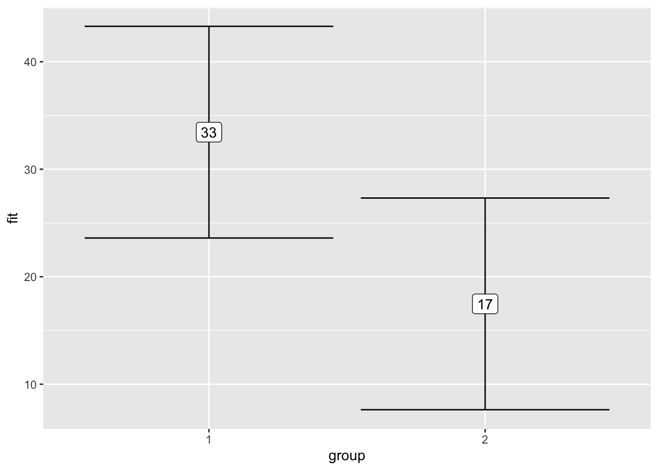

Data Visualization

You should always explore your data before running inferential statistics, based on your hypotheses. The inferential stats will confirm or refute your hypotheses.

Visualizations by Group

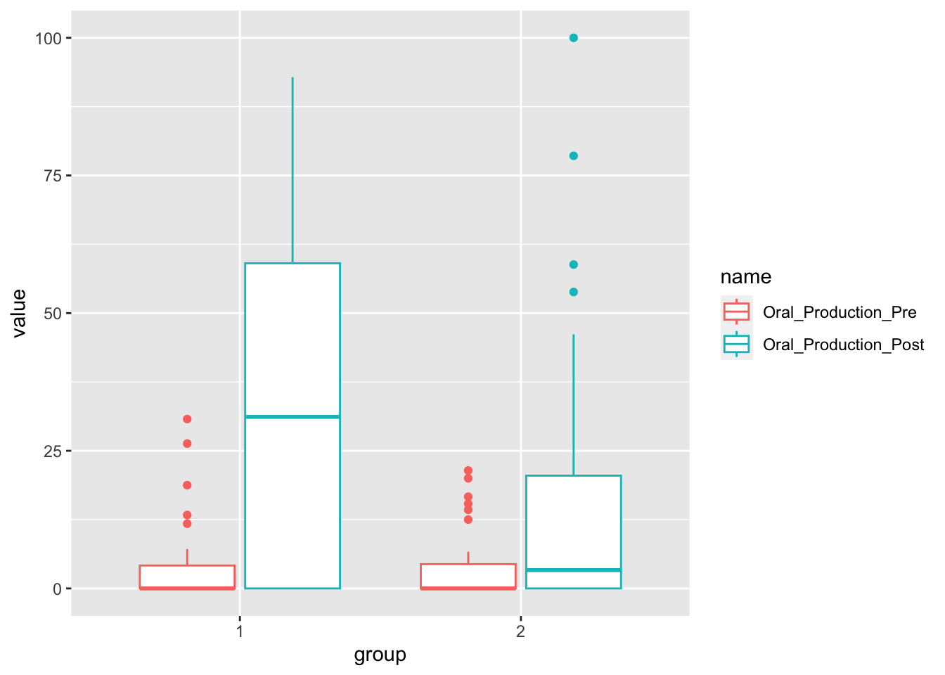
Oral production mean by group. We need to transform the data first, to have pre and post tests as values in a variable.

oral_production <- child_l2_data %>% 
  select(Participant, Group, Oral_Production_Pre, Oral_Production_Post) %>% 
  pivot_longer(cols = c(Oral_Production_Pre, Oral_Production_Post)) %>% 
  mutate(group = factor(Group),
         name = factor(name,
                       levels = c("Oral_Production_Pre",
                                  "Oral_Production_Post")))

We can now create a boxplot by group and type of test.

oral_production %>% 
  ggplot(aes(x = group,
             y = value,
             color = name)) +
  geom_boxplot()