Interactive Plots
Data
Download the Licensed Drivers by Sex and Age Groups, 1963 - 2023 data and set up your working environment.
Create a .qmd document so when we get to interactive documents, your plots will work.
- What questions can we answer with this data set?
- What plots can we create to answer these questions?
Histogram
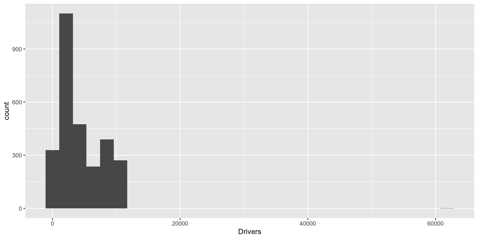
Scatter Plot
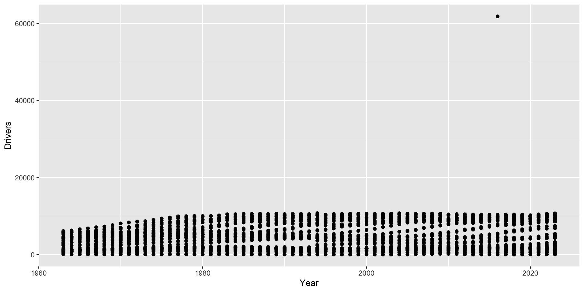
Compare different data sources
If we check the other version of this data set, we can clearly see the error.
Filter data
Scatter Plot
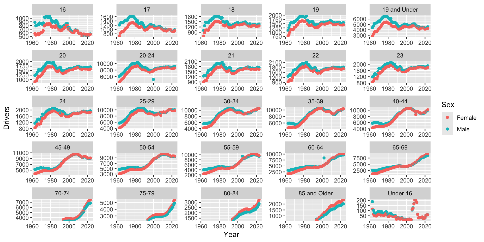
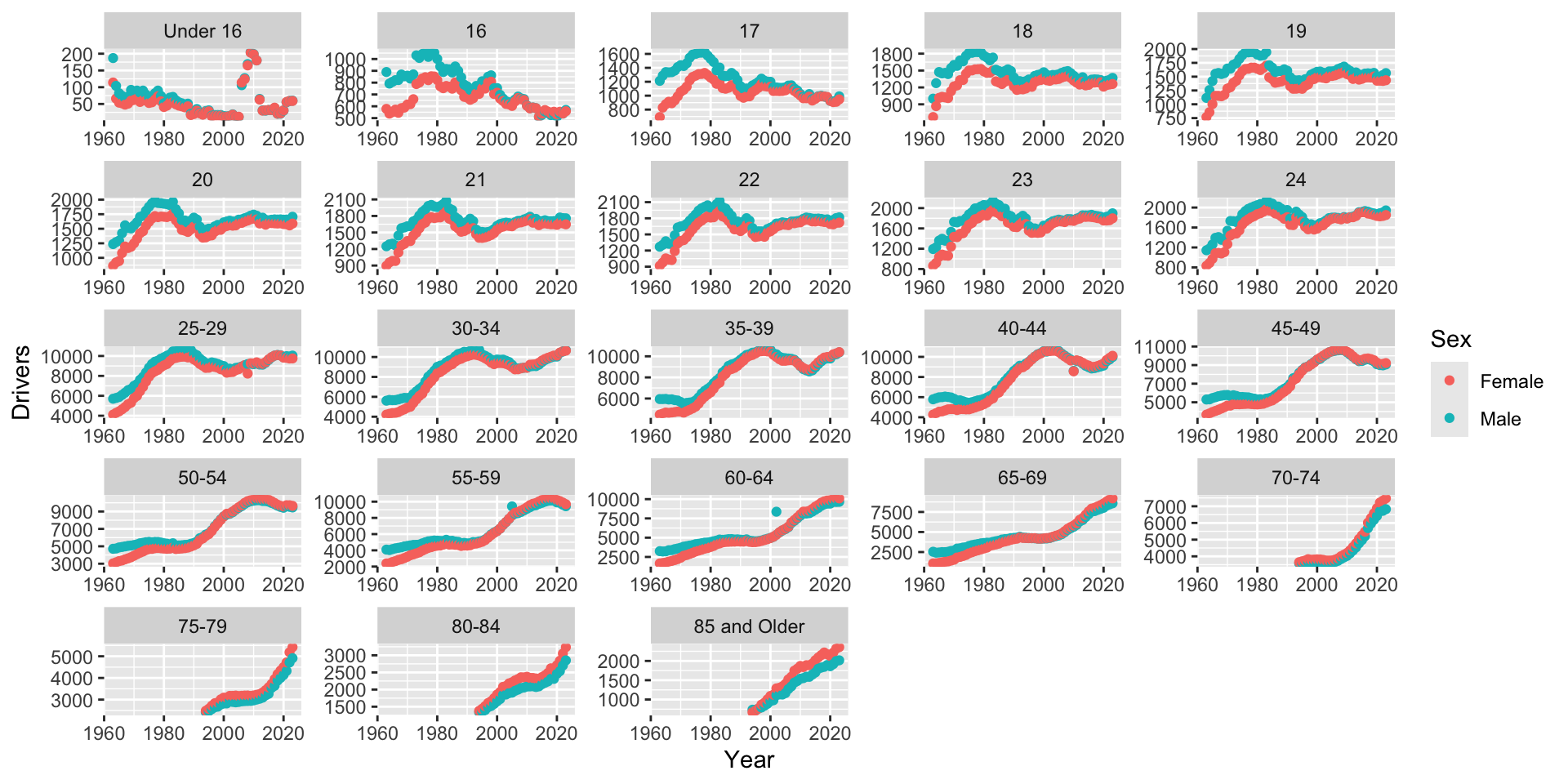
Ordered Categorical Variable
mutated_drivers <- mutated_drivers |>
  filter(Cohort != "19 and Under" &
           Cohort != "20-24") |>
  mutate(Cohort = factor(Cohort,
                         levels = c("Under 16",
                                    "16", "17", "18",
                                    "19", "20", "21", "22",
                                    "23", "24", "25-29",
                                    "30-34", "35-39","40-44",
                                    "45-49", "50-54", "55-59",
                                    "60-64", "65-69", "70-74",
                                    "75-79", "80-84", "85 and Older")))
Scatter Plot
Model
How has number of drivers (y) changed over time?
Call:
lm(formula = Drivers ~ Year + Cohort:Sex, data = mutated_drivers)

Residuals:
    Min      1Q  Median      3Q     Max
-2862.4  -786.2   -97.2   871.2  3387.9

Coefficients: (1 not defined because of singularities)
                               Estimate Std. Error t value Pr(>|t|)
(Intercept)                  -98261.519   2611.437 -37.627  < 2e-16 ***
Year                             49.612      1.296  38.274  < 2e-16 ***
CohortUnder 16:SexFemale       -562.990    248.891  -2.262 0.023783 *
Cohort16:SexFemale               52.846    248.891   0.212 0.831870
Cohort17:SexFemale              446.534    248.891   1.794 0.072918 .
Cohort18:SexFemale              666.551    248.891   2.678 0.007453 **
Cohort19:SexFemale              808.010    248.891   3.246 0.001184 **
Cohort20:SexFemale              881.830    248.891   3.543 0.000403 ***
Cohort21:SexFemale              938.223    248.891   3.770 0.000167 ***
Cohort22:SexFemale              985.551    248.891   3.960 7.71e-05 ***
Cohort23:SexFemale             1025.305    248.891   4.119 3.92e-05 ***
Cohort24:SexFemale             1050.649    248.891   4.221 2.52e-05 ***
Cohort25-29:SexFemale          7848.846    248.891  31.535  < 2e-16 ***
Cohort30-34:SexFemale          7803.715    248.891  31.354  < 2e-16 ***
Cohort35-39:SexFemale          7549.207    248.891  30.331  < 2e-16 ***
Cohort40-44:SexFemale          7143.961    248.891  28.703  < 2e-16 ***
Cohort45-49:SexFemale          6709.518    248.891  26.958  < 2e-16 ***
Cohort50-54:SexFemale          6194.879    248.891  24.890  < 2e-16 ***
Cohort55-59:SexFemale          5534.846    248.891  22.238  < 2e-16 ***
Cohort60-64:SexFemale          4690.272    248.891  18.845  < 2e-16 ***
Cohort65-69:SexFemale          3703.895    248.891  14.882  < 2e-16 ***
Cohort70-74:SexFemale          3363.200    287.242  11.709  < 2e-16 ***
Cohort75-79:SexFemale          2084.900    287.242   7.258 5.20e-13 ***
Cohort80-84:SexFemale           847.500    287.242   2.950 0.003202 **
Cohort85 and Older:SexFemale    222.767    287.242   0.776 0.438096
CohortUnder 16:SexMale         -553.613    248.891  -2.224 0.026216 *
Cohort16:SexMale                153.846    248.891   0.618 0.536548
Cohort17:SexMale                609.977    248.891   2.451 0.014322 *
Cohort18:SexMale                853.452    248.891   3.429 0.000616 ***
Cohort19:SexMale                996.174    248.891   4.002 6.45e-05 ***
Cohort20:SexMale               1043.223    248.891   4.191 2.87e-05 ***
Cohort21:SexMale               1081.731    248.891   4.346 1.44e-05 ***
Cohort22:SexMale               1122.600    248.891   4.510 6.77e-06 ***
Cohort23:SexMale               1158.272    248.891   4.654 3.43e-06 ***
Cohort24:SexMale               1177.338    248.891   4.730 2.37e-06 ***
Cohort25-29:SexMale            8423.125    248.891  33.843  < 2e-16 ***
Cohort30-34:SexMale            8242.075    248.891  33.115  < 2e-16 ***
Cohort35-39:SexMale            7904.698    248.891  31.760  < 2e-16 ***
Cohort40-44:SexMale            7491.944    248.891  30.101  < 2e-16 ***
Cohort45-49:SexMale            7067.387    248.891  28.396  < 2e-16 ***
Cohort50-54:SexMale            6560.108    248.891  26.357  < 2e-16 ***
Cohort55-59:SexMale            5915.846    248.891  23.769  < 2e-16 ***
Cohort60-64:SexMale            5066.928    248.891  20.358  < 2e-16 ***
Cohort65-69:SexMale            3977.026    248.891  15.979  < 2e-16 ***
Cohort70-74:SexMale            3121.967    287.242  10.869  < 2e-16 ***
Cohort75-79:SexMale            1823.167    287.242   6.347 2.59e-10 ***
Cohort80-84:SexMale             610.467    287.242   2.125 0.033662 *
Cohort85 and Older:SexMale           NA         NA      NA       NA
---
Signif. codes:  0 '***' 0.001 '**' 0.01 '*' 0.05 '.' 0.1 ' ' 1

Residual standard error: 1112 on 2511 degrees of freedom
  (248 observations deleted due to missingness)
Multiple R-squared:  0.8885,    Adjusted R-squared:  0.8864
F-statistic: 434.9 on 46 and 2511 DF,  p-value: < 2.2e-16
Effects
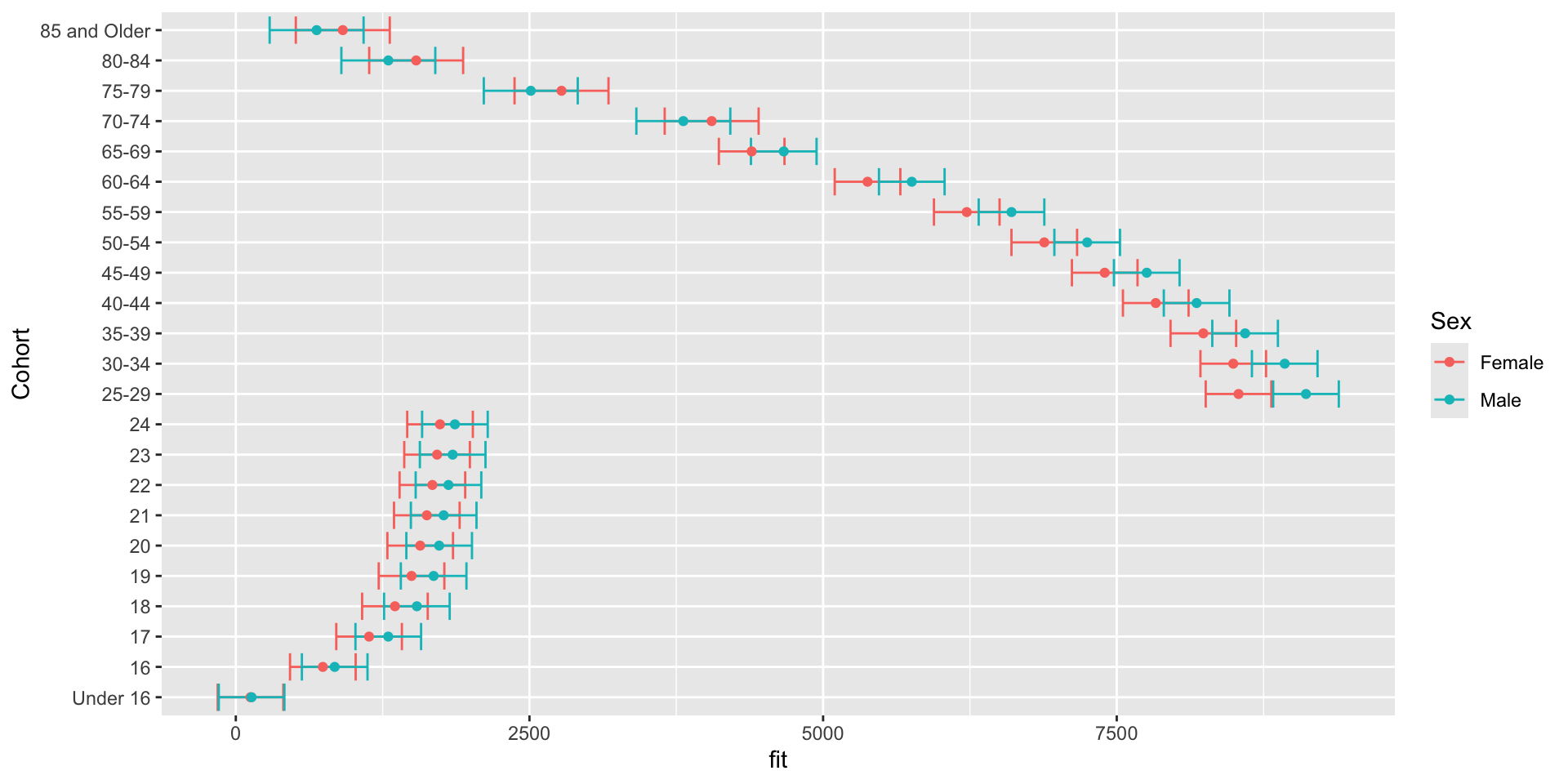
Interactive Plot – code
Interactive Plot – plot
Scatter Plot
Case Study
Download the number of drivers per state data and plot an interactive map.