Plotting Maps

Data

Download the data on average cost of undergraduate student by state USA and set up your working environment. Make sure all columns names are lowercased.

library(tidyverse)
library(janitor)

college_cost <- read_csv("data/nces330_20.csv") |>
  clean_names()

Questions

What affects college cost?

How does college cost vary by state?

Modeling the data

We will run linear regression with value as our response variable, and the other variables are predictors

model <- lm(value ~ state + year + expense + type + length,
            data = college_cost)
summary(model)


Call:
lm(formula = value ~ state + year + expense + type + length, 
    data = college_cost)

Residuals:
   Min     1Q Median     3Q    Max 
-14624  -3355   -488   3134  19403 

Coefficients:
                            Estimate Std. Error t value Pr(>|t|)    
(Intercept)               -8.996e+05  6.459e+04 -13.927  < 2e-16 ***
stateAlaska               -4.559e+02  8.421e+02  -0.541 0.588306    
stateArizona              -1.668e+02  8.164e+02  -0.204 0.838139    
stateArkansas             -1.129e+03  8.164e+02  -1.383 0.166797    
stateCalifornia            3.834e+03  8.164e+02   4.696 2.75e-06 ***
stateColorado              2.154e+03  8.164e+02   2.639 0.008352 ** 
stateConnecticut           6.072e+03  8.164e+02   7.438 1.28e-13 ***
stateDelaware              1.502e+03  8.495e+02   1.768 0.077065 .  
stateDistrict of Columbia  1.834e+03  1.007e+03   1.820 0.068845 .  
stateFlorida              -6.634e+00  8.164e+02  -0.008 0.993517    
stateGeorgia               1.200e+03  8.164e+02   1.470 0.141581    
stateHawaii                1.162e+03  8.164e+02   1.423 0.154864    
stateIdaho                -2.754e+03  8.164e+02  -3.373 0.000752 ***
stateIllinois              3.805e+03  8.164e+02   4.661 3.27e-06 ***
stateIndiana               2.704e+03  8.164e+02   3.312 0.000936 ***
stateIowa                  1.041e+03  8.164e+02   1.275 0.202341    
stateKansas               -7.733e+02  8.164e+02  -0.947 0.343598    
stateKentucky              1.579e+03  8.164e+02   1.934 0.053239 .  
stateLouisiana             1.993e+03  8.164e+02   2.441 0.014691 *  
stateMaine                 3.016e+03  8.164e+02   3.695 0.000224 ***
stateMaryland              3.970e+03  8.164e+02   4.863 1.21e-06 ***
stateMassachusetts         5.919e+03  8.164e+02   7.251 5.07e-13 ***
stateMichigan              2.519e+03  8.164e+02   3.086 0.002046 ** 
stateMinnesota             1.280e+03  8.164e+02   1.567 0.117113    
stateMississippi          -1.706e+03  8.164e+02  -2.089 0.036756 *  
stateMissouri             -1.880e+02  8.164e+02  -0.230 0.817894    
stateMontana               2.962e+02  8.164e+02   0.363 0.716745    
stateNebraska             -6.609e+02  8.164e+02  -0.810 0.418234    
stateNevada                8.436e+02  8.351e+02   1.010 0.312505    
stateNew Hampshire         5.198e+03  8.164e+02   6.367 2.18e-10 ***
stateNew Jersey            4.496e+03  8.164e+02   5.507 3.90e-08 ***
stateNew Mexico           -1.248e+03  8.164e+02  -1.529 0.126366    
stateNew York              3.921e+03  8.164e+02   4.802 1.63e-06 ***
stateNorth Carolina        1.481e+03  8.164e+02   1.814 0.069718 .  
stateNorth Dakota         -2.135e+03  8.164e+02  -2.615 0.008955 ** 
stateOhio                  2.258e+03  8.164e+02   2.766 0.005705 ** 
stateOklahoma             -1.475e+02  8.164e+02  -0.181 0.856623    
stateOregon                4.171e+03  8.164e+02   5.109 3.41e-07 ***
statePennsylvania          5.006e+03  8.164e+02   6.132 9.63e-10 ***
stateRhode Island          5.339e+03  8.164e+02   6.540 7.06e-11 ***
stateSouth Carolina        2.084e+03  8.164e+02   2.553 0.010727 *  
stateSouth Dakota         -1.716e+03  8.164e+02  -2.102 0.035661 *  
stateTennessee             2.120e+03  8.164e+02   2.597 0.009437 ** 
stateTexas                 1.234e+03  8.164e+02   1.511 0.130841    
stateUtah                 -2.444e+03  8.164e+02  -2.994 0.002773 ** 
stateVermont               7.234e+03  8.164e+02   8.861  < 2e-16 ***
stateVirginia              2.825e+03  8.164e+02   3.460 0.000546 ***
stateWashington            3.367e+03  8.164e+02   4.125 3.80e-05 ***
stateWest Virginia        -1.282e+03  8.164e+02  -1.571 0.116294    
stateWisconsin             1.137e+03  8.164e+02   1.392 0.163906    
stateWyoming              -1.676e+03  8.615e+02  -1.946 0.051760 .  
year                       4.508e+02  3.202e+01  14.079  < 2e-16 ***
expenseRoom/Board         -9.711e+03  1.886e+02 -51.475  < 2e-16 ***
typePublic In-State       -8.319e+03  2.219e+02 -37.496  < 2e-16 ***
typePublic Out-of-State   -2.061e+03  2.194e+02  -9.394  < 2e-16 ***
length4-year               1.229e+04  2.234e+02  55.015  < 2e-16 ***
---
Signif. codes:  0 '***' 0.001 '**' 0.01 '*' 0.05 '.' 0.1 ' ' 1

Residual standard error: 4864 on 3492 degrees of freedom
Multiple R-squared:  0.6947,    Adjusted R-squared:  0.6899 
F-statistic: 144.5 on 55 and 3492 DF,  p-value: < 2.2e-16

Effect of state in our model

Let’s save the effect of state to a data frame, so we can plot the results:

library(effects)

by_state <- effect("state", model) |>
  data.frame()

Plotting a map

First we need to load the usmap library (run install.packages("usmap") to install it).

library(usmap)

Then we can plot our results:

plot_usmap(data = by_state, 
           values = "fit")

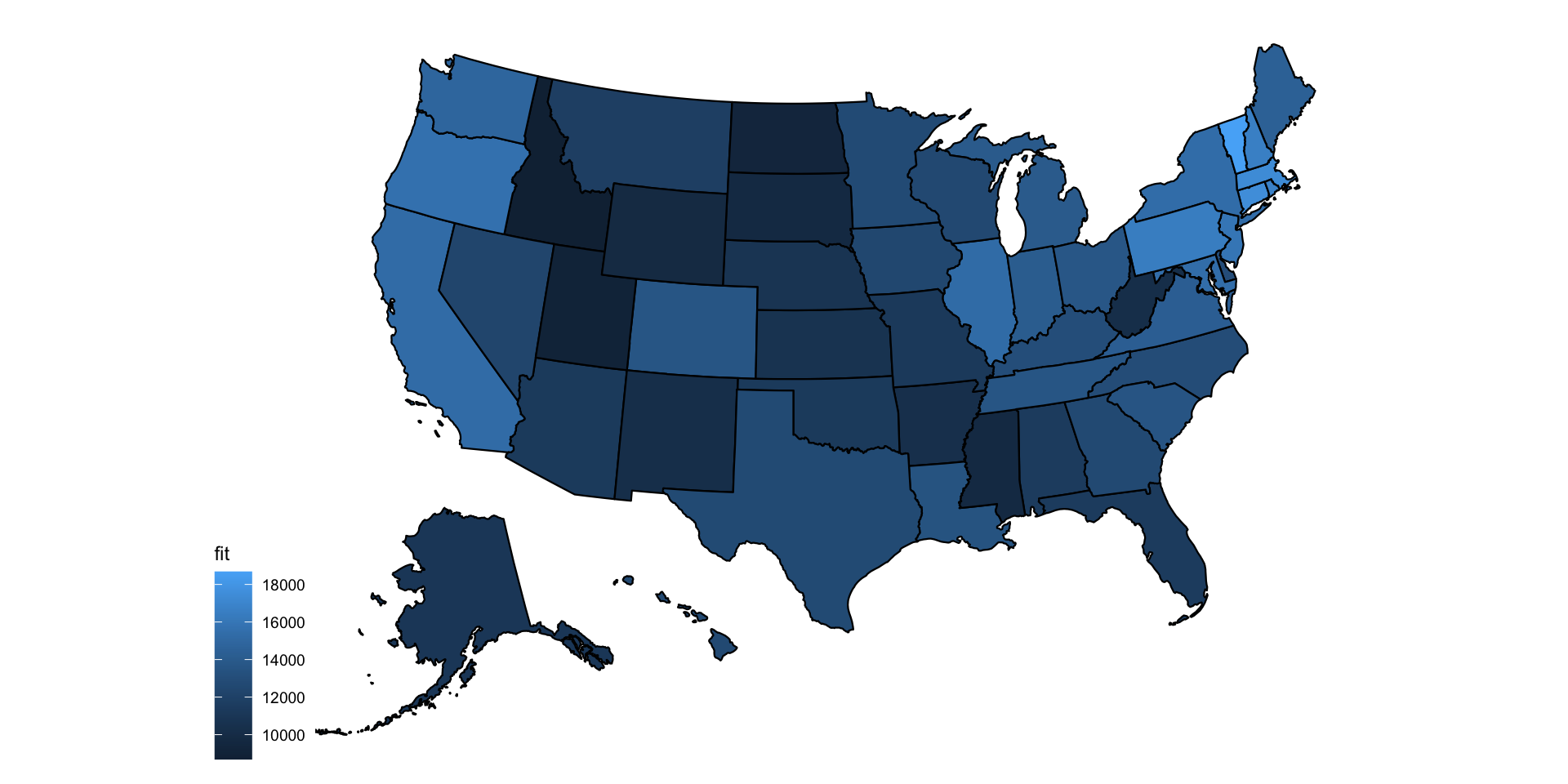
What issues do we have with this plot?

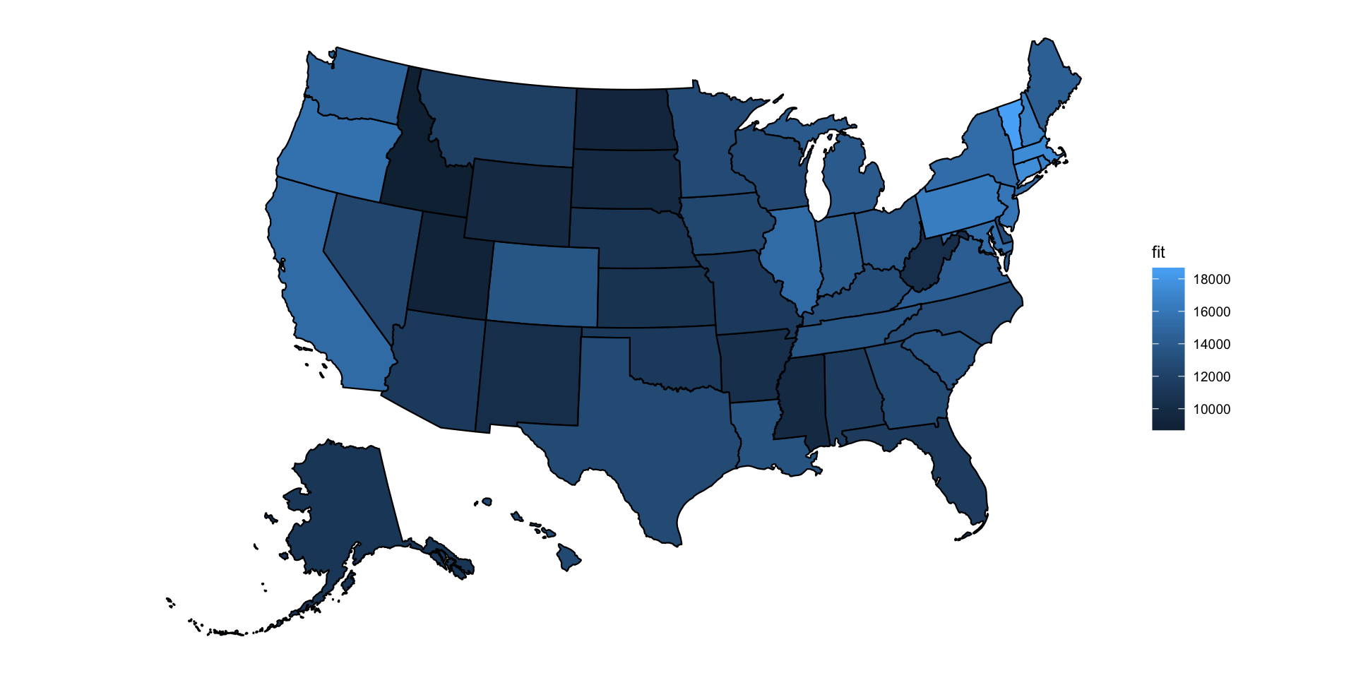
Improving our map plot

We can move the legend to the right:

plot_usmap(data = by_state, 
           values = "fit") +
  theme(legend.position = "right")

Improving our map plot

We can add a light color for low numbers, and a dark color for high values:

plot_usmap(data = by_state, 
           values = "fit") +
  theme(legend.position = "right") +
  scale_fill_continuous(name = "US Dollars",
                        low = "#dcfae7", 
                        high = "#005721")

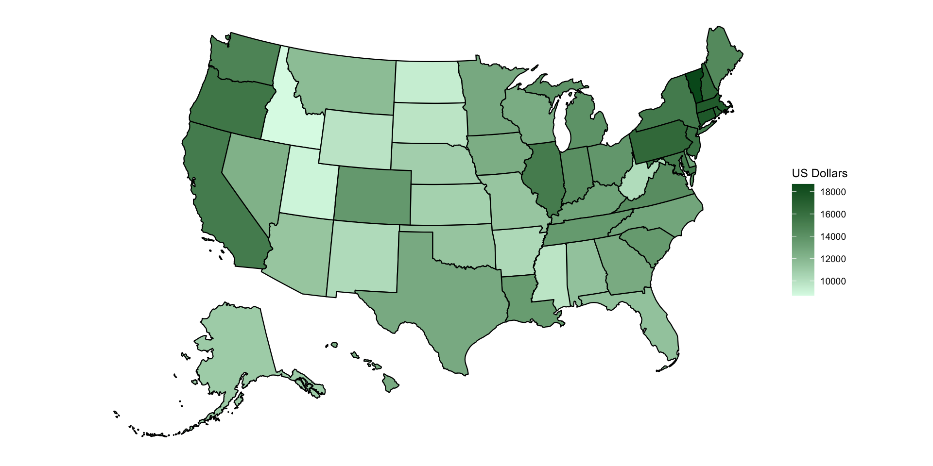
Improving our map plot

We can add a title:

plot_usmap(data = by_state, 
           values = "fit") +
  theme(legend.position = "right") +
  scale_fill_continuous(name = "US Dollars",
                        low = "#dcfae7", 
                        high = "#005721") +
  labs(title = "Average college cost in US dollars")

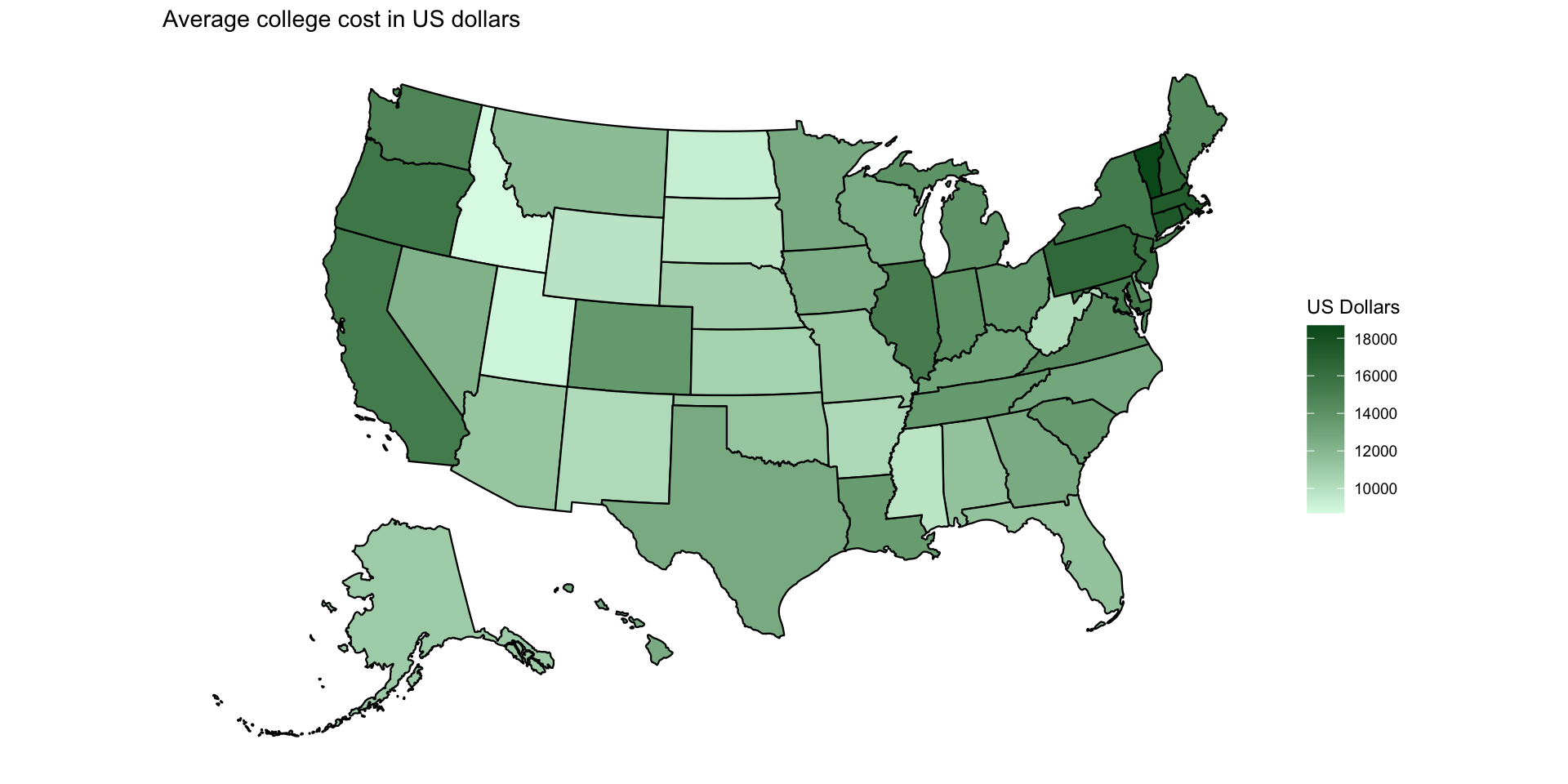
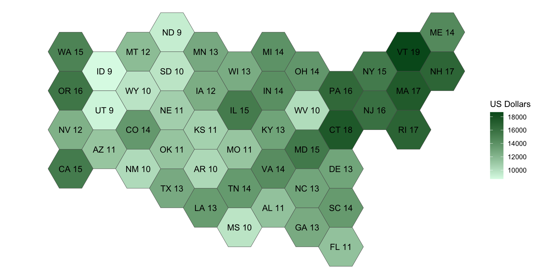
Improving our map plot

Adding labels – we need to get centroids first.

centroid_labels <- usmapdata::centroid_labels("states") |>
  rename("state" = full)
by_state_labels <- merge(centroid_labels, by_state, by = "state")

Then we plot it:

plot_usmap(data = by_state_labels, 
           values = "fit") +
  theme(legend.position = "right") +
  scale_fill_continuous(name = "US Dollars",
                        low = "#dcfae7", 
                        high = "#005721") +
  geom_sf_text(aes(label = round(fit/1000))) +
  labs(title = "Average college cost in thousands of US dollars")

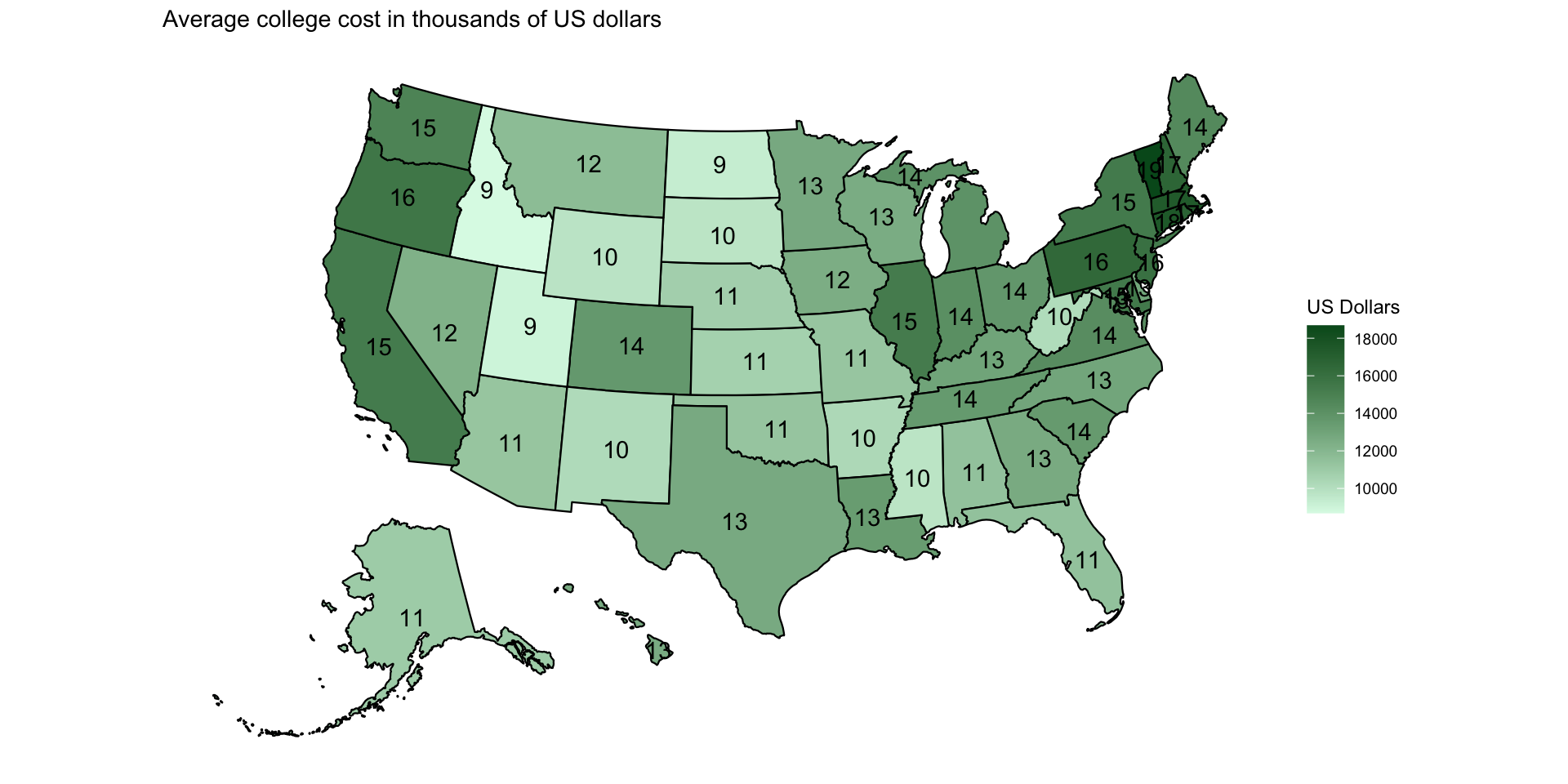
Improving our map plot

plot_usmap(data = by_state, 
           values = "fit", include = c("MA", "CT", "RI", "NJ", "NY", "PA")) +
  theme(legend.position = "right") +
  scale_fill_continuous(name = "US Dollars",
                        low = "#dcfae7", 
                        high = "#005721") +
  geom_sf_text(aes(label = round(fit/1000))) +
  labs(title = "Average college cost in thousands of US dollars")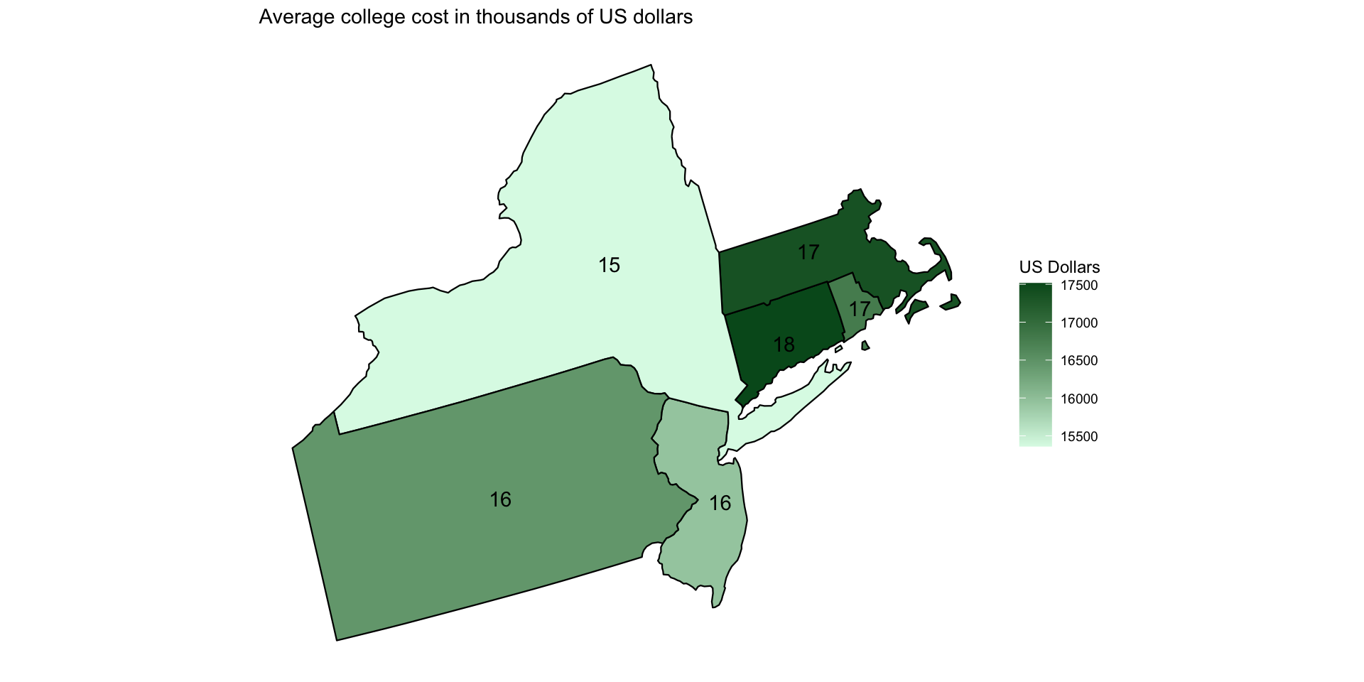

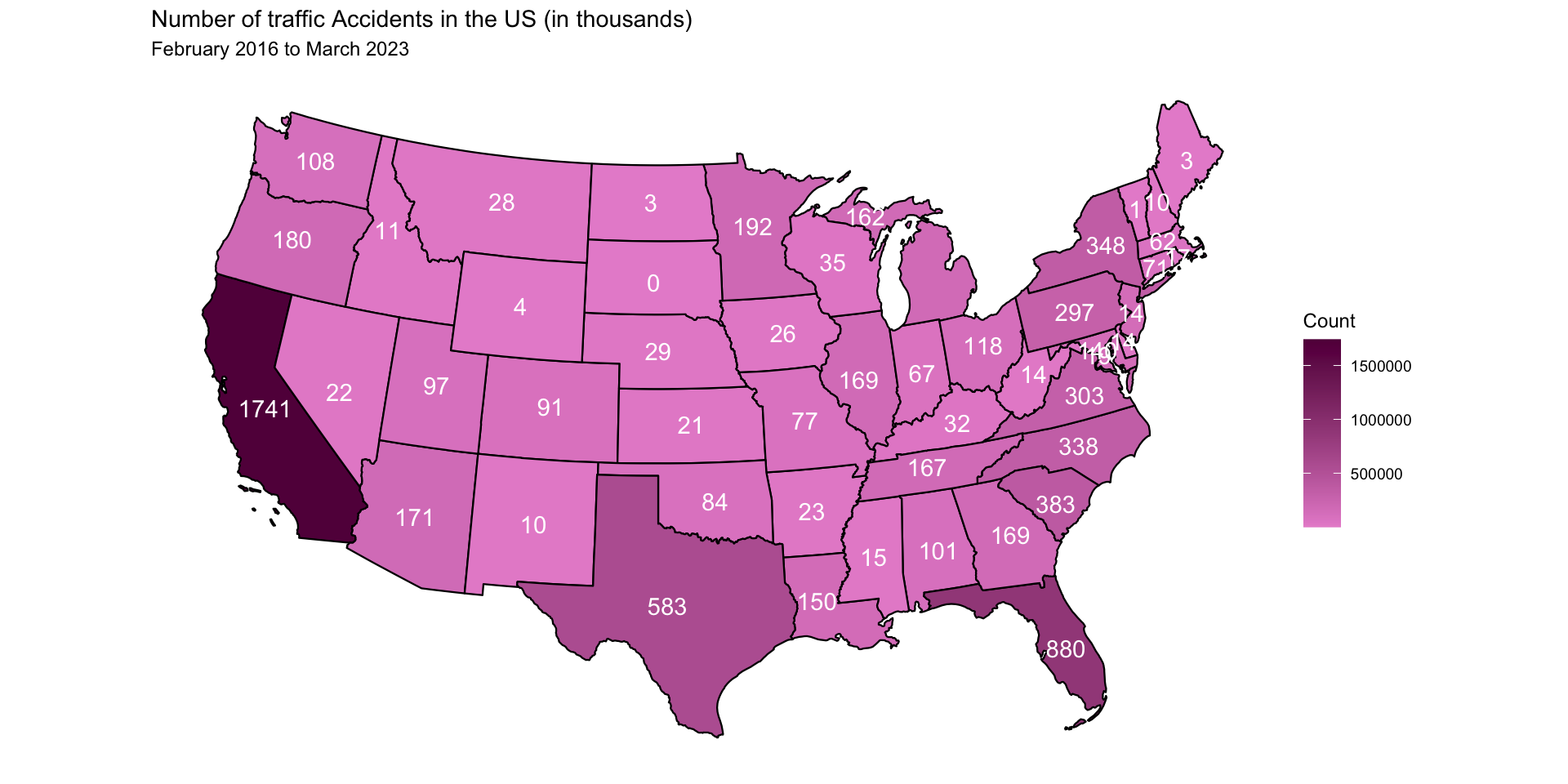
Case study

US breweries

Case Study

US accidents

Tile maps

library(tilemaps)
library(sf)

full_data <- governors |>
  mutate(tile_map = generate_map(geometry, square = FALSE, flat_topped = TRUE))  |>
  full_join(statepop, by = join_by(abbreviation == abbr)) |>
  rename("state" = full) 

full_data <- by_state |>
  left_join(full_data)

full_data |> 
  ggplot(aes(geometry = tile_map, label = paste(abbreviation,round(fit/1000)),
             fill = fit)) +
  geom_sf() +
  geom_sf_text(fun.geometry = function(x) st_centroid(x)) +
  scale_fill_continuous(name = "US Dollars",
                        low = "#dcfae7", 
                        high = "#005721") +
  theme_void()

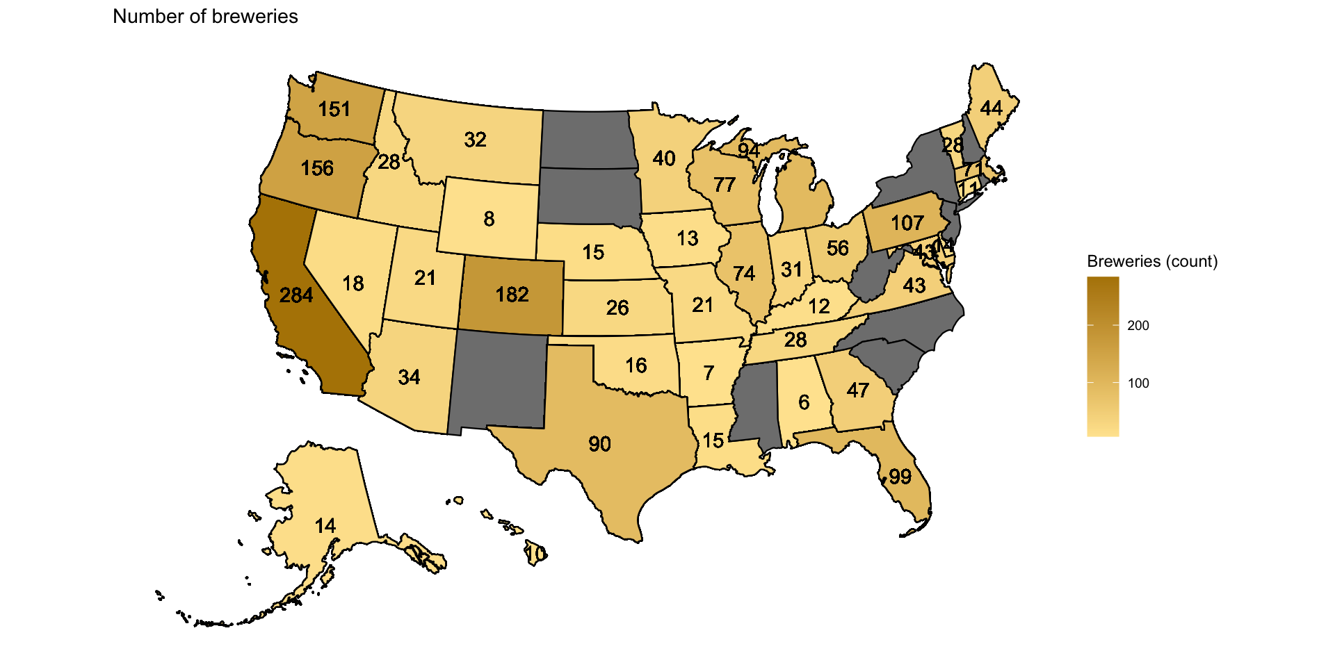
Tile maps

World Map

world <- map_data("world")

world %>%
  ggplot(aes(x = long,
               y = lat,
               map_id = region)) + 
  geom_map(map = world)

Gapminder

Different indicators per country