Review
Dependent variable: Rating
Step 1: Histogram
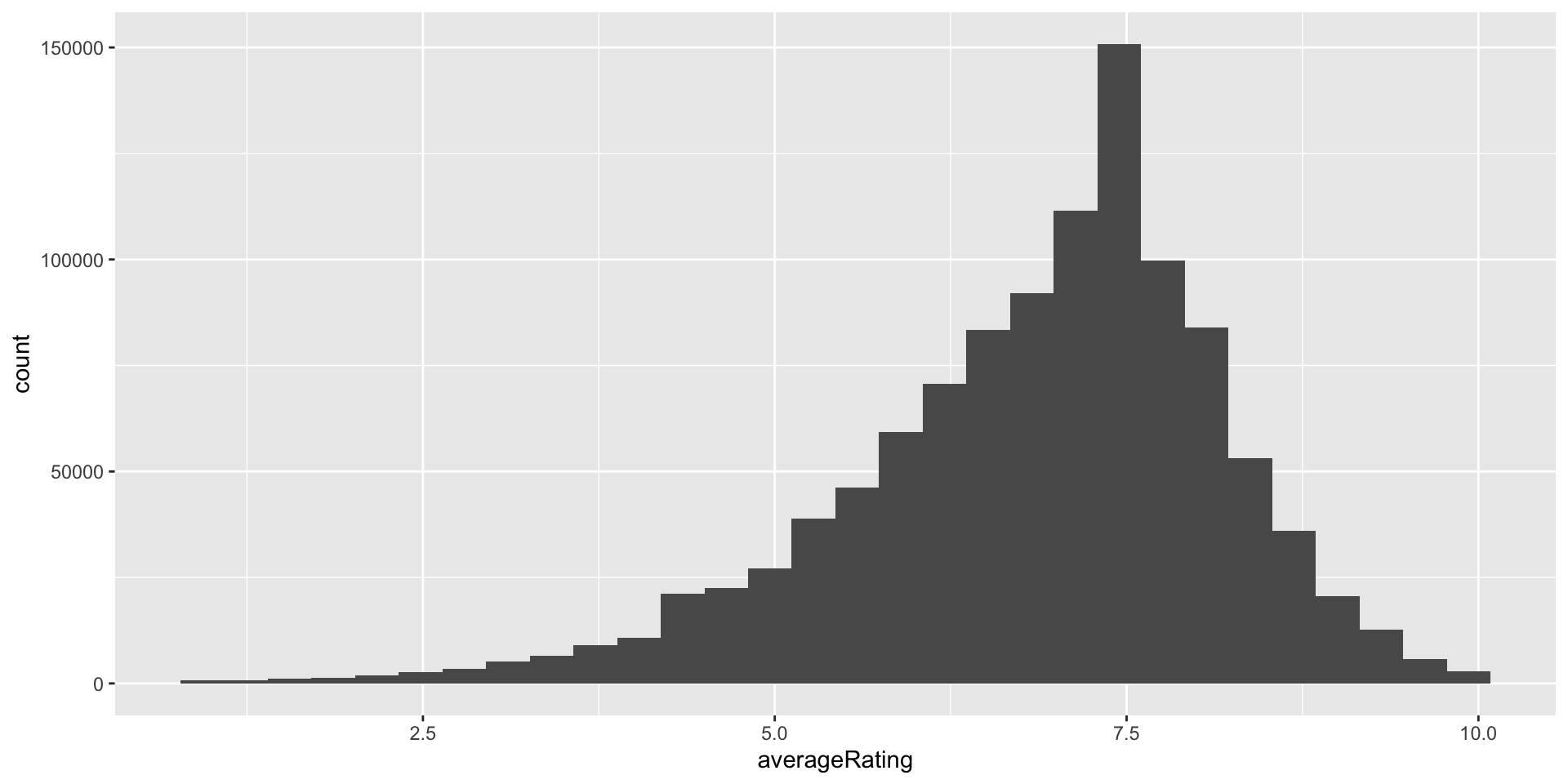
What can we say about the distribution of the rating variable?
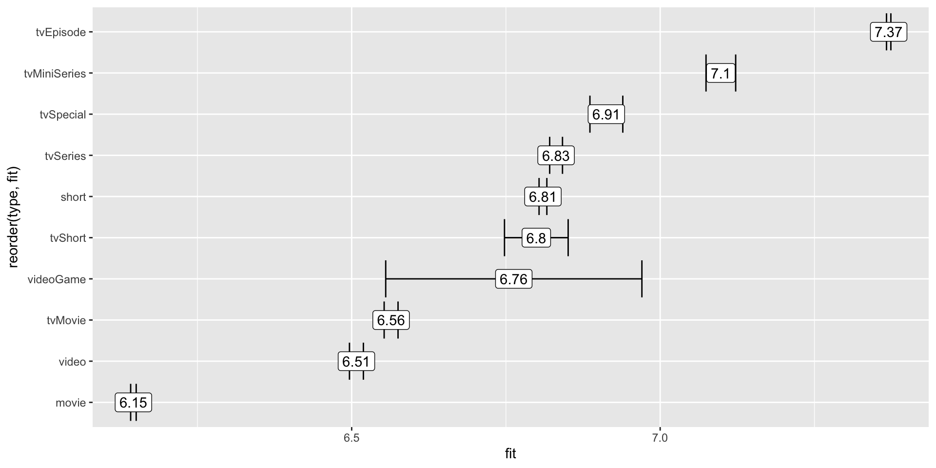
Independent variable: type
Boxplot
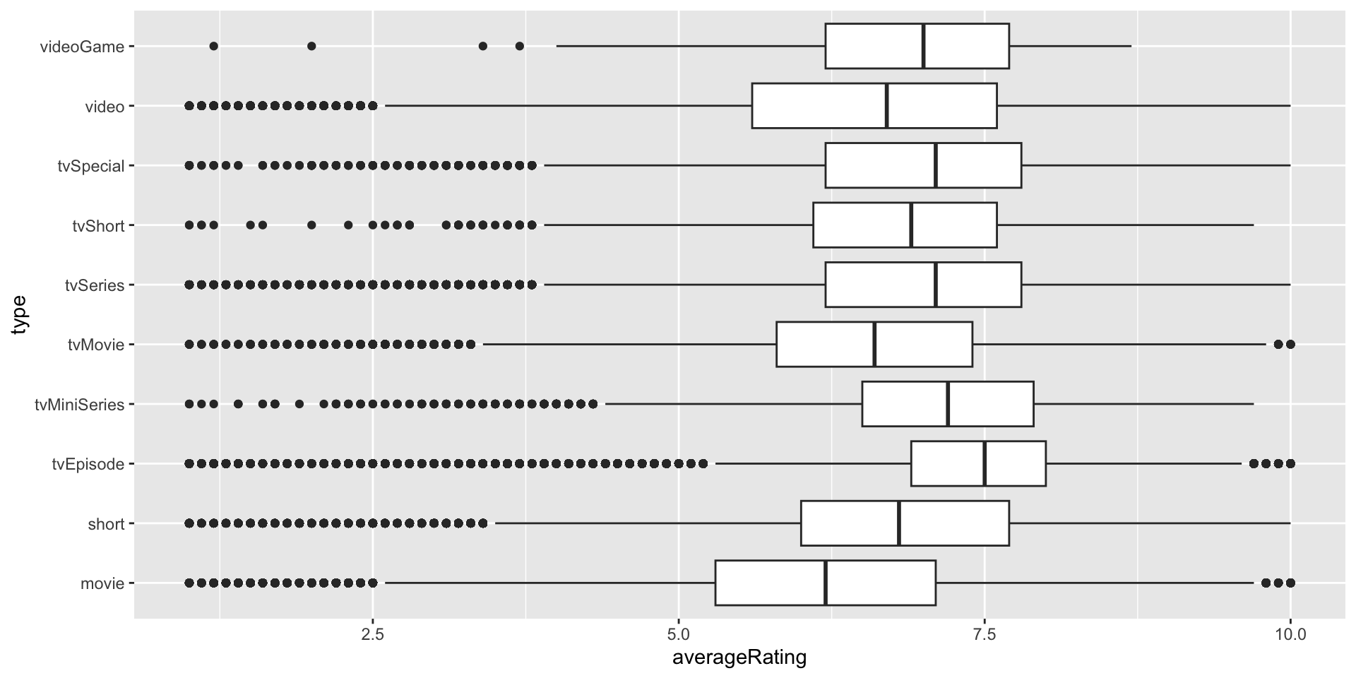
Rating vs. Type
What is the effect of type on rating?
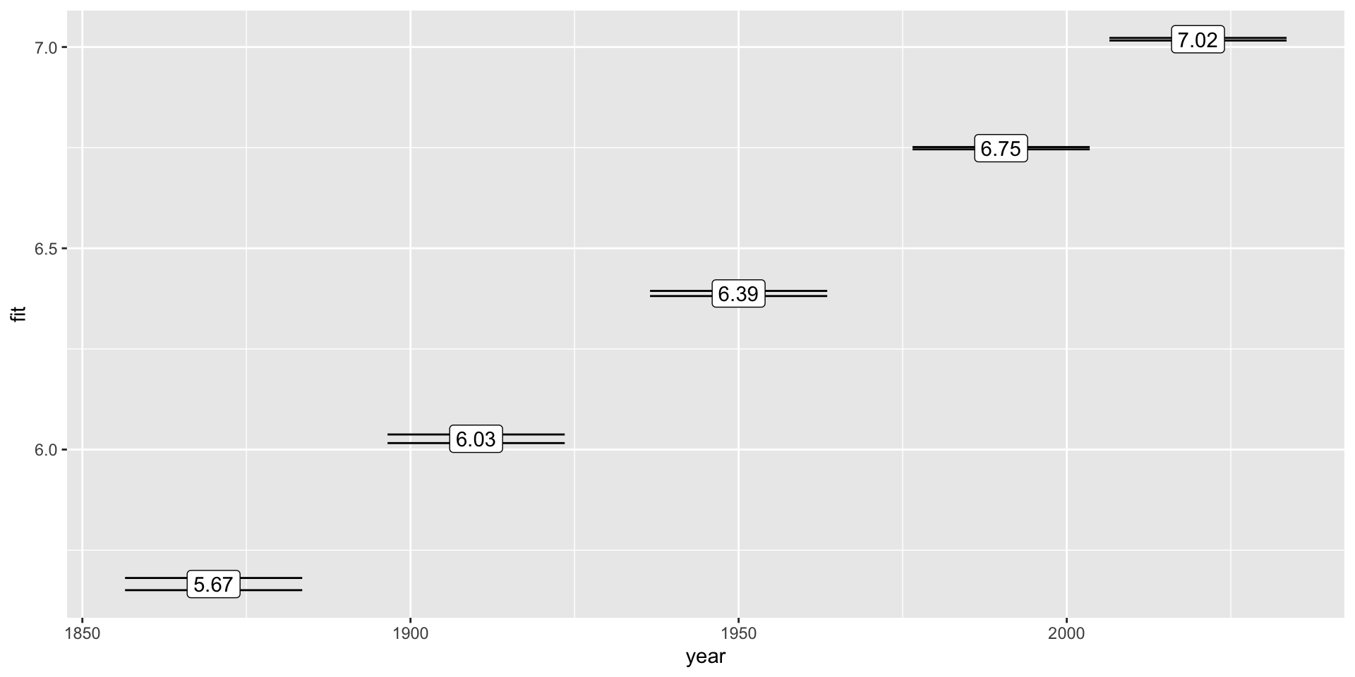
Independent variable: year
Scatter plot
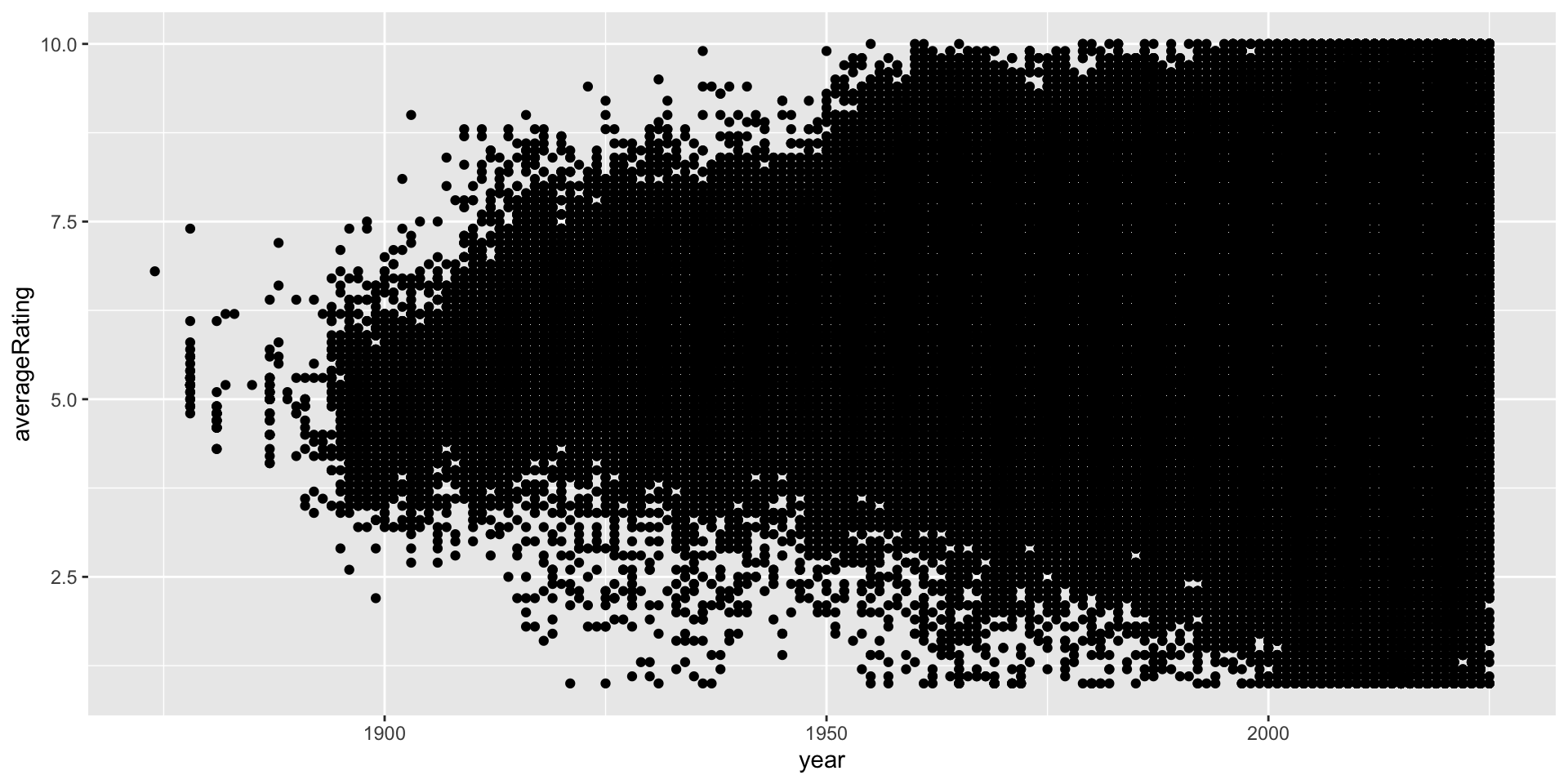
Rating vs. Year
What is the effect of year on rating?