Bivariate Analysis

Two numeric variables

We saw two hypothesis tests for checking if differences in the mean of a numeric variable across different groups is real (t-test and ANOVA)

What if we have two numeric variables?

scatterplots
correlation
linear regression

Case Study

We will be working with Indicators of Anxiety or Depression Based on Reported Frequency of Symptoms in November 2020-2024

Please download the clean data and set up your analysis environment.

library(tidyverse)
dep_anx <- read_csv("data/depression-anxiety.csv")

Question

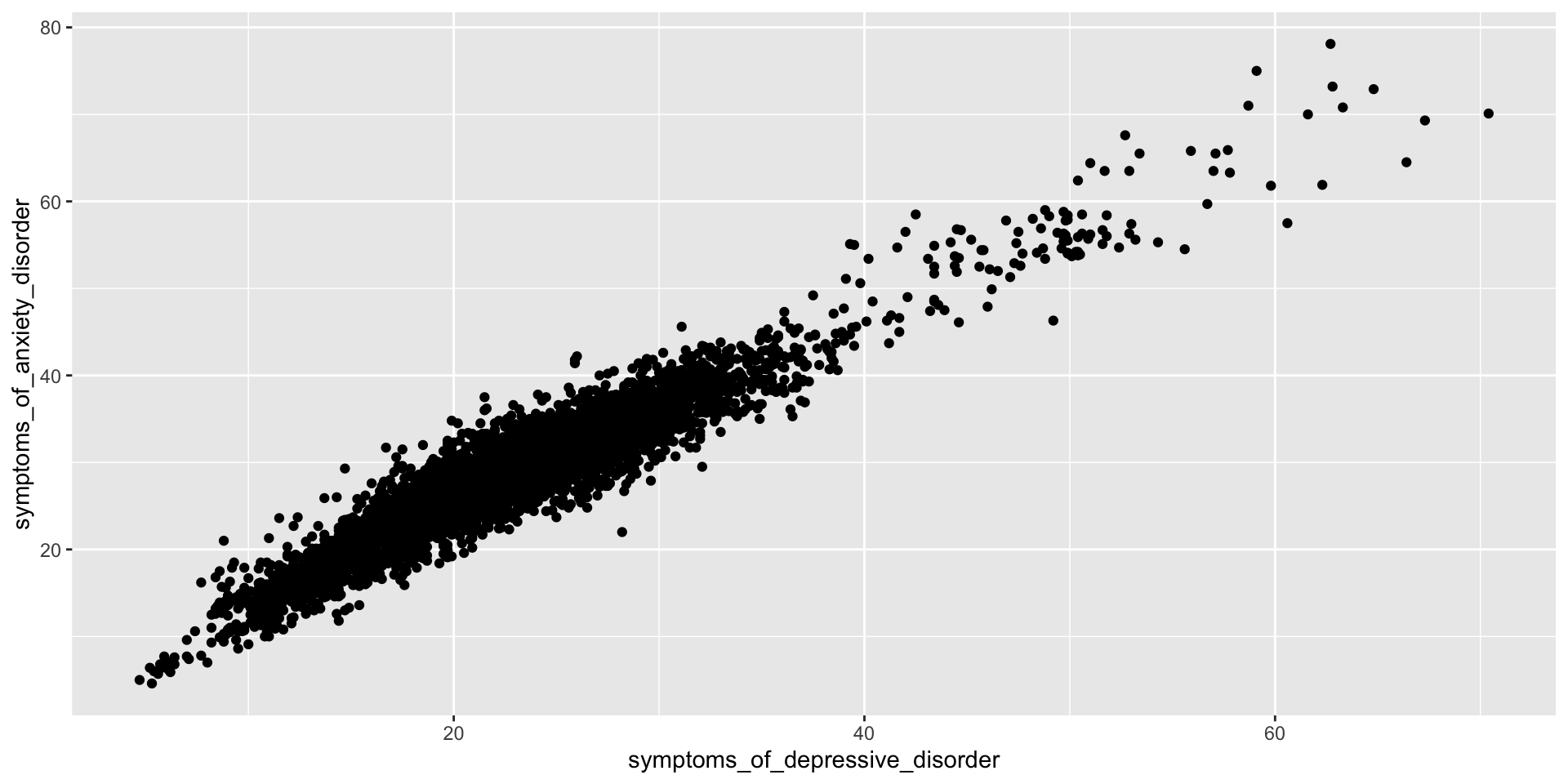
Does reported frequency of anxiety symptoms correlate with reported frequency of depression symptoms?

Descriptive Statistics – Scatterplot

dep_anx |>
  ggplot(aes(x = symptoms_of_depressive_disorder,
             y = symptoms_of_anxiety_disorder)) +
  geom_point()

Association – Correlation

evaluates the association between two or more numeric variables
when one variable changes, does the other variable change along with it?
correlation coefficient ranges from -1 to +1:
- +1 means a perfect positive correlation (as one increases, the other increases)
- -1 means a perfect negative correlation (as one increases, the other decreases)
- 0 means no correlation (the variables don’t appear related)

Null and Alternative Hypotheses

\(H_0\): There is no linear relationship between frequency of anxiety and frequency of depression

\(H_1\): There is a linear relationship between frequency of anxiety and frequency of depression

Pearson correlation formula

\(r = \frac{\sum_{i=1}^n (x_i - \bar{x})*(y_i - \bar{y})}{\sqrt{\sum_{i=1}^n (x_i - \bar{x})^2*\sum_{i=1}^n(y_i - \bar{y})^2}}\)

Where:

x and y are two vectors of length n
\(\bar{x}\) and \(\bar{y}\) are the means of x and y, respectively

Association – Correlation

We use cor.test() to calculate correlation in R.

cor.test(dep_anx$symptoms_of_depressive_disorder,
         dep_anx$symptoms_of_anxiety_disorder)


    Pearson's product-moment correlation

data:  dep_anx$symptoms_of_depressive_disorder and dep_anx$symptoms_of_anxiety_disorder
t = 219.22, df = 5359, p-value < 2.2e-16
alternative hypothesis: true correlation is not equal to 0
95 percent confidence interval:
 0.9457571 0.9511318
sample estimates:
      cor 
0.9485127

Questions

What other questions can you answer with this data set?

One numeric and one categorical variable

Is reported frequency of symptoms of depressive disorder higher in transgender than cis-gender people?

by_gender <- dep_anx |>
  filter(group == "By Gender identity") 

by_gender |>
  count(subgroup)

subgroup	n
Cis-gender female	44
Cis-gender male	44
Transgender	44

Recoding variable

by_gender <- by_gender|>
  mutate(transgender = if_else(subgroup == "Transgender",
                               "yes", "no"))

by_gender |>
  count(subgroup, transgender)

subgroup	transgender	n
Cis-gender female	no	44
Cis-gender male	no	44
Transgender	yes	44

Two-way t-test

What’s the Null Hypothesis?

t.test(symptoms_of_depressive_disorder ~ transgender,
       data = by_gender)


    Welch Two Sample t-test

data:  symptoms_of_depressive_disorder by transgender
t = -26.835, df = 46.646, p-value < 2.2e-16
alternative hypothesis: true difference in means between group no and group yes is not equal to 0
95 percent confidence interval:
 -38.12833 -32.80919
sample estimates:
 mean in group no mean in group yes 
         19.61282          55.08158

Since the p-value is lower than the alpha of 0.05, we can reject the null hypothesis.

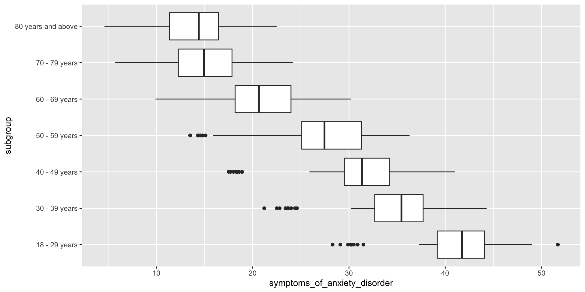
Anxiety by Age

Is reported frequency of sympoms of anxiety different across age groups?

by_age <- dep_anx |>
  filter(group == "By Age")

Anova

What’s the Null Hypothesis?

anova <- aov(symptoms_of_anxiety_disorder ~ subgroup, data = by_age)
summary(anova)

             Df Sum Sq Mean Sq F value Pr(>F)    
subgroup      6  45677    7613     290 <2e-16 ***
Residuals   497  13047      26                   
---
Signif. codes:  0 '***' 0.001 '**' 0.01 '*' 0.05 '.' 0.1 ' ' 1
70 observations deleted due to missingness

Since the p-value is lower than the alpha of 0.05, we can reject the null hypothesis.

Box Plot

by_age |>
  ggplot(aes(x = symptoms_of_anxiety_disorder,
             y = subgroup)) +
  geom_boxplot()