Exploring Categorical Data

Descriptive Statistics

• distribution (histogram)
• central tendency (mean, median, mode)
• variability (range, standard deviation, variance, interquartile range – IQR)

Data

We will be working with the same US demographic data for our exploratory analyses.

You can download the csv file and add it to your RStudio (or Posit Cloud) project if you have not done that yet.

Create a new R script file and save it as county-categorical-data-analysis.R and load the tidyverse package and the data.

library(tidyverse)
county <- read_csv("data/county.csv")

Distribution – adding categorical variable

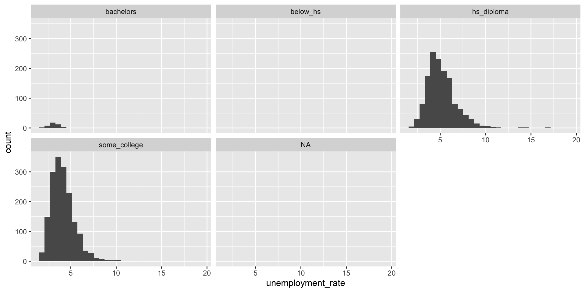
Histogram: the frequency distribution of a continuous variable across different groups

county |>
  ggplot(aes(x = unemployment_rate)) + 
  geom_histogram() +
  facet_wrap(~median_edu)

Inspect categorical variable

county |>
  count(median_edu)

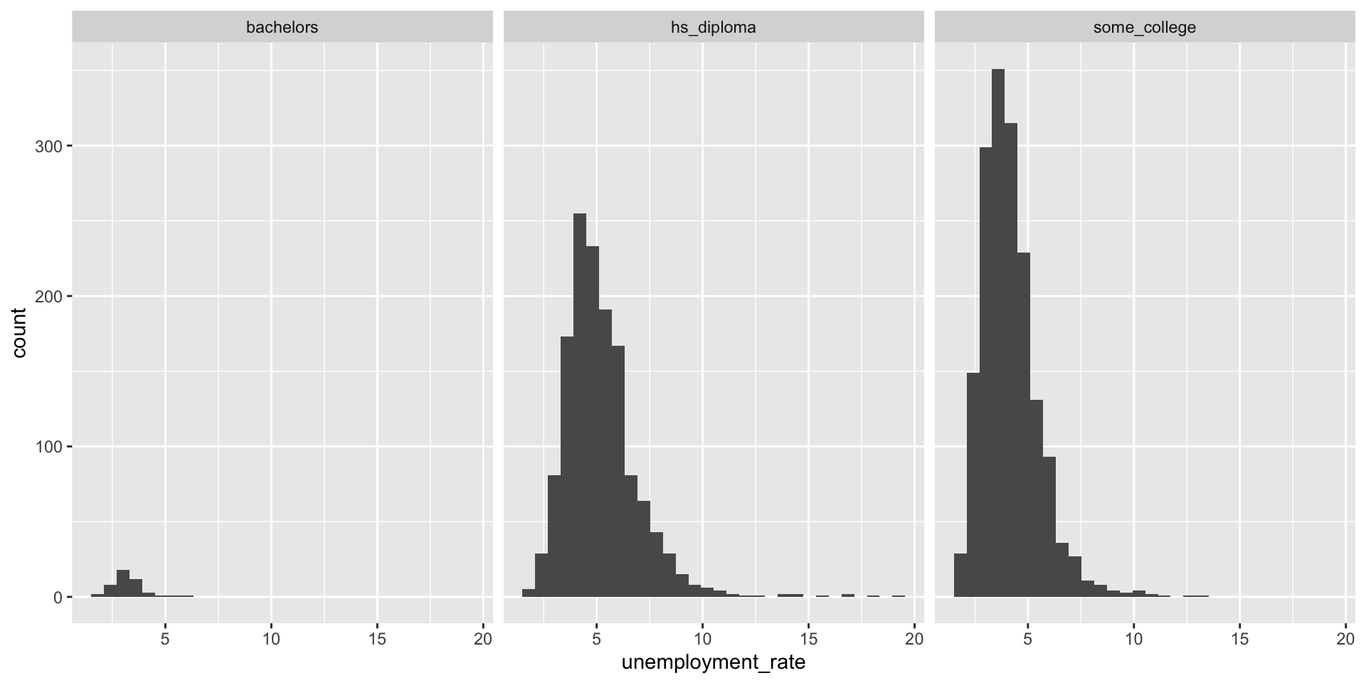
Distribution – with filtered data

county |>
  filter(median_edu != "below_hs",
         !is.na(median_edu)) |>
  ggplot(aes(x = unemployment_rate)) + 
  geom_histogram() +
  facet_wrap(~median_edu)

Measures of Central Tendency

Mean and median – add group_by with categorical variable

county |>
  group_by(median_edu) |>
  summarize(mean = mean(unemployment_rate, na.rm = TRUE),
            median = median(unemployment_rate, na.rm = TRUE))

Variability

Range, standard deviation – add group_by with categorical variable

county |>
  group_by(median_edu) |>
  summarize(min = min(unemployment_rate, na.rm = TRUE),
            max = max(unemployment_rate, na.rm = TRUE),
            sd = sd(unemployment_rate, na.rm = TRUE)) |>
  mutate(range = max - min)

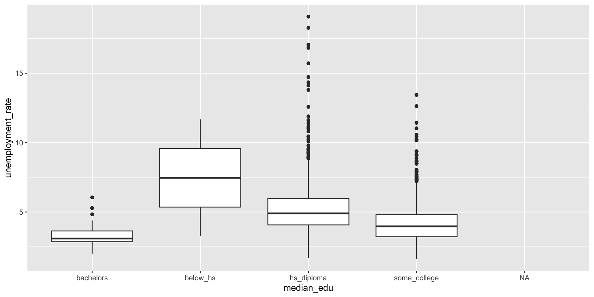
Variability – Box plot (IQR)

county |>
  ggplot(aes(y = unemployment_rate,
             x = median_edu)) +
  geom_boxplot()