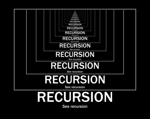
Recursion

CSCI 1913 – Introduction to Algorithms, Data Structures, and Program Development
Adriana Picoral

Recursion is Magic

To write a recursive function, you need to believe that it already works (but only for a smaller version of the same problem).
Sometimes that step is called the “recursive leap of faith”

What is recursion?

In general? Something defined in terms of itself
In Computer Science? A recursive function that calls itself
An alternative to loops

Recursion inside recursion inside recursion inside recursion inside…

Recursion vs. Loops

Loops are easier to understand conceptually
Loops are generally faster
In many problems, loops will be fewer lines of code
Anything you can do with recursion, you can do with loops (and vice versa)
So why use recursion?

Recursively Defined Problems

There are some problems where the recursive solution is significantly less code, easier to understand, and requires fewer constructs.
These are generally problems where the problem structure is tree-like in nature
- For example, visiting all nodes in a binary tree in-order, you recursively visit the left subtree, process the current node, then recursively visit the right subtree.

Function Stacks

Some programming languages use what is called a function stack
A function stack is a data structure that holds a function name, arguments, and a return point for functions
A new function adds to the stack building up
Python does not require function stacks, but the implementation we are all likely using “CPython” is implemented using function stacks

Function Stacks

What will this print?

def fun_a():
  print("A")
  fun_b()
  print("Another A")
  
def fun_b():
  print("B")
  
def fun_c():
  print("C")
  
if __name__ == "__main__":
  fun_a()
  fun_b()
  fun_c()

A
B
Another A
B
C

Remember factorial?

What’s the runtime?

def factorial(n):
  product = 1
  while n > 0:
    product *= n
    n -= 1
  return product

if __name__ == "__main__":
  assert factorial(1) == 1
  assert factorial(5) == 120
  assert factorial(7) == 5040

Remember factorial?

What’s the runtime? \(O(n)\)

def factorial(n):
  product = 1
  while n > 0:
    product *= n
    n -= 1
  return product

if __name__ == "__main__":
  assert factorial(1) == 1
  assert factorial(5) == 120
  assert factorial(7) == 5040

Recursive factorial

“a recursive function calls itself”

def factorial(n):
  factorial(n)

“Infinite” Recursion

Happens when your recursive steps never reach a base case
Each time you call a function, memory is allocated to remember things like what it was called with, what line it’s currently at, variables, etc. (Function stack in Cpython)
Python limits how deep the stack can get to avoid memory problems (maximum recursion depth)

You must have at least one Base Case

The First Law of Recursion

Recursive factorial

“a recursive function must have at least one base case”

What’s our base case for our recursive factorial function?

Recursive factorial

“a recursive function needs a base case”

def factorial(n):
  if n == 1:
    return 1
  factorial(n)

Base Case

Directly return the solution for that specific case
Do not have a recursive call
Are generally a “trivial solution”

Your Recursive Case(s) must always move towards a Base Case

The Second Law of Recursion

Recursive factorial

“recursive case(s) must always move towards a base case”

What’s our recursive case for our factorial function?

Recursive factorial

“recursive case(s) must always mode towards a base case”

We need to get to 1

def factorial(n):
  if n == 1:
    return 1
  factorial(n-1)

Recursive factorial

a recursive function needs at lease one base case
recursive case(s) must always mode towards a base case
it needs to provide the correct answer

\(5! = 5 * 4 * 3 * 2 * 1\)

For various math reasons, \(0!\) is defined to be \(1\)

Recursive factorial

def factorial(n):
  if n == 1 or n == 0:
    return 1
  return n*factorial(n-1)

if __name__ == "__main__":
  assert factorial(1) == 1
  assert factorial(5) == 120

Recurrence relations

The runtime complexity T(N) of a recursive function will have function T on both sides of the equation

single recursive call \(T(N-1)\)
one multiplication of the result \(O(1)\)

def factorial(n):
  if n == 1 or n == 0:
    return 1
  return n*factorial(n-1)

Using O-notation to express runtime complexity of a recursive function requires solving the recurrence relation.

Recurrence relations

single recursive call \(T(n-1)\)
one multiplication of the result \(O(1)\)

def factorial(n):
  if n == 1 or n == 0:
    return 1
  return n*factorial(n-1)

\(T(N) = T(N-1) + 1\)

Recurrence relations

\(T(N) = T(N-1) + 1\)

def factorial(n):
  if n == 1 or n == 0:
    return 1
  return n*factorial(n-1)

\(T(0) = 1\)
\(T(1) = 1\) base case
\(T(2) = T(1) + 1 = 1 + 1 = 2\)
\(T(3) = T(2) + 1 = 2 + 1 = 3\)
\(T(4) = T(3) + 1 = 3 + 1 = 4\)
\(T(N) = N\)

Recurrence relations – Recursive Factorial

\(T(N) = T(N-1) + 1\)
\(T(N-1) = T(N-2) + 1\)
\(T(N) = T(N-2) + 1 + 1\)
\(T(N) = T(N-3) + 1 + 1 + 1\)
\(T(N) = T(N-4) + 1 + 1 + 1 + 1\)

…

Recurrence relations – Recursive Factorial

\(T(N) = T(0) + N\)
\(T(N) = 1 + N\)
\(T(N) = N\)

How to Write a Recursive Function

Construct at least one base case (more may be needed if there are inputs that won’t eventually reach that base case).
Find a recurrence relation: a solution expressed in terms of the solution to a smaller instance of the same problem.
Pretend that your function magically works for the smaller instance of the problem, use this to construct the recursive case

Exercise – Binary Search

Here’s our original Binary Search implementation:

def binary_search(arr, v):
  low = 0
  high = len(arr)-1
  while low <= high:
    mid = (low+high) // 2
    if v > arr[mid]: # update low
      low = mid + 1
    elif v < arr[mid]: # update high
      high = mid - 1
    else:
      return mid
  return -1

if __name__ == "__main__":
  numbers = [0, 5, 10, 23, 41, 43, 44, 60, 99, 120, 343]
  assert binary_search(numbers, 99) == 8
  assert binary_search(numbers, 9) == -1

Exercise – Binary Search

Write binary search as a recursive function.

What are the base cases?
What’s the recursive case?

Remember:

a recursive function needs at lease one base case
recursive case(s) must always mode towards a base case
it needs to provide the correct answer

Exercise – Binary Search

Write binary search as a recursive function.

What are the base case? low > high
What’s the recursive case? n/2 – divide list by two or change either low or high

Call your function binary_search and your file binary_search.py to submit to gradescope